[ ] 说明TensorFlow的数据流图结构
[ ] 应用TensorFlow操作图
[ ] 说明会话在TensorFlow中的作用
[ ] 应用TensorFlow实现张量的创建、形状类型修改操作
[ ] 应用Variable实现变量op的操作
[ ] 应用tensorboard实现图结构以及张量值的显示
[ ] 应用tf.train.saver实现TensorFlow的模型保存以及加载
[ ] 应用tf.app.flags实现命令行参数的添加和使用
[ ] 应用TensorFlow实现线性回归
一 基础入门 1.1 快速启动 使用TensorFlow实现一个简单的加法运算
import tensorflow as tftf.compat.v1.disable_eager_execution() def add () : """ TensorFlow的基本结构 :return: """ a_t = tf.constant(2 ) b_t = tf.constant(3 ) c_t = a_t + b_t print("\n" ) print(" TensorFlow 加法运算的结果为 " , c_t) print("\n" ) with tf.compat.v1.compat.v1.Session() as sess: c_t_val = sess.run(c_t) print(" TensorFlow 加法运算的结果 c_t 的真实值为 " , c_t_val) if __name__ == "__main__" : add()
运行结果如下
TensorFlow 加法运算的结果为 Tensor("add:0" , shape=(), dtype=int32) TensorFlow 加法运算的结果 c_t 的真实值为 5
TensorFlow程序通常被组织为一个构件图阶段和一个执行图阶段
一个构建图阶段
在构建阶段,数据与操作的执行步骤被描述为一个图
在执行阶段,使用会话执行构建好的图中的操作
图和会话
图: 这是TensorFlow将计算表示为指令之间的依赖关系的一种表示法
会话:TensorFlow跨一个或多个本地或远程设备运行数据流图的机制
张量:TensorFlow中的基本数据对象
节点:提供图当中执行的操作
TensorFlow是一个采用数据流图,用于数值计算的框架
节点(Operation)在图中表示数学操作,线(edges)则表示在节点间相互联系的多维数据数组,即张量(tensor)
1.2 图相关的操作 1.2.1 默认图操作 通常TensorFlow会默认帮我们创建一张图
查看默认图的两种方法
通过调用get_default_graph()访问,要将操作添加到默认图形中,直接创建op即可
op和sess都含有graph属性,默认都在一张图中
import tensorflow as tftf.compat.v1.disable_eager_execution() t = tf.compat.v1.compat.v1 def add () : a_t = t.constant(2 ) b_t = t.constant(3 ) c_t = a_t + b_t print(" TensorFlow 加法运算的结果为 " , c_t) default_graph = t.get_default_graph() print(" default_graph = " , default_graph) print(" a_t 的图属性 = " , a_t.graph) print(" b_t 的图属性 = " , b_t.graph) print(" c_t 的图属性 = " , c_t.graph) with t.Session() as sess: c_t_val = sess.run(c_t) print(" TensorFlow 加法运算的结果 c_t 的真实值为 " , c_t_val) print(" sess 的图属性 = " , sess.graph) if __name__ == "__main__" : add()
运行结果为
TensorFlow 加法运算的结果为 Tensor("add:0" , shape=(), dtype=int32) default_graph = <tensorflow.python.framework.ops.Graph object at 0x0000017EB5092CD0 > a_t 的图属性 = <tensorflow.python.framework.ops.Graph object at 0x0000017EB5092CD0 > b_t 的图属性 = <tensorflow.python.framework.ops.Graph object at 0x0000017EB5092CD0 > c_t 的图属性 = <tensorflow.python.framework.ops.Graph object at 0x0000017EB5092CD0 > TensorFlow 加法运算的结果 c_t 的真实值为 5 sess 的图属性 = <tensorflow.python.framework.ops.Graph object at 0x0000017EB5092CD0 >
1.2.2 创建图 可以通过Graph()自定义创建图
如果要在这张图中创建OP,典型的用法是使用Graph.as_default()上下文管理器
import tensorflow as tftf.compat.v1.disable_eager_execution() t = tf.compat.v1.compat.v1 def add () : a_t = t.constant(2 ) b_t = t.constant(3 ) c_t = a_t + b_t print(" TensorFlow 加法运算的结果为 " , c_t) default_graph = t.get_default_graph() print(" default_graph = " , default_graph) print(" a_t 的图属性 = " , a_t.graph) print(" b_t 的图属性 = " , b_t.graph) print(" c_t 的图属性 = " , c_t.graph) with t.Session() as sess: c_t_val = sess.run(c_t) print(" TensorFlow 加法运算的结果 c_t 的真实值为 " , c_t_val) print(" sess 的图属性 = " , sess.graph) new_g = t.Graph() with new_g.as_default(): a_new = t.constant(20 ) b_new = t.constant(30 ) c_new = a_new + b_new print(" c_new = " , c_new) if __name__ == "__main__" : add()
运行结果如下
TensorFlow 加法运算的结果为 Tensor("add:0" , shape=(), dtype=int32) default_graph = <tensorflow.python.framework.ops.Graph object at 0x00000241749E9310 > a_t 的图属性 = <tensorflow.python.framework.ops.Graph object at 0x00000241749E9310 > b_t 的图属性 = <tensorflow.python.framework.ops.Graph object at 0x00000241749E9310 > c_t 的图属性 = <tensorflow.python.framework.ops.Graph object at 0x00000241749E9310 > TensorFlow 加法运算的结果 c_t 的真实值为 5 sess 的图属性 = <tensorflow.python.framework.ops.Graph object at 0x00000241749E9310 > c_new = Tensor("add:0" , shape=(), dtype=int32)
对于以下代码,试图运行自定义图中的数据和操作
import tensorflow as tftf.compat.v1.disable_eager_execution() t = tf.compat.v1.compat.v1 def add () : a_t = t.constant(2 ) b_t = t.constant(3 ) c_t = a_t + b_t print(" TensorFlow 加法运算的结果为 " , c_t) default_graph = t.get_default_graph() print(" default_graph = " , default_graph) print(" a_t 的图属性 = " , a_t.graph) print(" b_t 的图属性 = " , b_t.graph) print(" c_t 的图属性 = " , c_t.graph) new_g = t.Graph() with new_g.as_default(): a_new = t.constant(20 ) b_new = t.constant(30 ) c_new = a_new + b_new print(" c_new = " , c_new) with t.Session() as sess: c_t_val = sess.run(c_t) print(" TensorFlow 加法运算的结果 c_t 的真实值为 " , c_t_val) print(" sess 的图属性 = " , sess.graph) c_new_val = sess.run(c_new) print(" TensorFlow 加法运算的结果 c_new_val 的真实值为 " , c_new_val) if __name__ == "__main__" : add()
运行结果出现异常
Traceback (most recent call last): File "<input>" , line 1 , in <module> File "C:\Program Files\JetBrains\PyCharm 2021.1.1\plugins\python\helpers\pydev\_pydev_bundle\pydev_umd.py" , line 197 , in runfile pydev_imports.execfile(filename, global_vars, local_vars) File "C:\Program Files\JetBrains\PyCharm 2021.1.1\plugins\python\helpers\pydev\_pydev_imps\_pydev_execfile.py" , line 18 , in execfile exec(compile(contents+"\n" , file, 'exec' ), glob, loc) File "F:/python_workspace/atguigu/graph_demo.py" , line 44 , in <module> add() File "F:/python_workspace/atguigu/graph_demo.py" , line 39 , in add c_new_val = sess.run(c_new) File "F:\python_workspace\atguigu\venv\lib\site-packages\tensorflow\python\client\session.py" , line 967 , in run result = self._run(None , fetches, feed_dict, options_ptr, File "F:\python_workspace\atguigu\venv\lib\site-packages\tensorflow\python\client\session.py" , line 1175 , in _run fetch_handler = _FetchHandler( File "F:\python_workspace\atguigu\venv\lib\site-packages\tensorflow\python\client\session.py" , line 487 , in __init__ self._fetch_mapper = _FetchMapper.for_fetch(fetches) File "F:\python_workspace\atguigu\venv\lib\site-packages\tensorflow\python\client\session.py" , line 278 , in for_fetch return _ElementFetchMapper(fetches, contraction_fn) File "F:\python_workspace\atguigu\venv\lib\site-packages\tensorflow\python\client\session.py" , line 313 , in __init__ raise ValueError('Fetch argument %r cannot be interpreted as a ' ValueError: Fetch argument <tf.Tensor 'add:0' shape=() dtype=int32> cannot be interpreted as a Tensor. (Tensor Tensor("add:0" , shape=(), dtype=int32) is not an element of this graph.)
这是因为对于接口Session()在默认情况下使用的是默认图
修改代码为以下
import tensorflow as tftf.compat.v1.disable_eager_execution() t = tf.compat.v1.compat.v1 def add () : a_t = t.constant(2 ) b_t = t.constant(3 ) c_t = a_t + b_t print(" TensorFlow 加法运算的结果为 " , c_t) default_graph = t.get_default_graph() print(" default_graph = " , default_graph) print(" a_t 的图属性 = " , a_t.graph) print(" b_t 的图属性 = " , b_t.graph) print(" c_t 的图属性 = " , c_t.graph) new_g = t.Graph() with new_g.as_default(): a_new = t.constant(20 ) b_new = t.constant(30 ) c_new = a_new + b_new print(" c_new = " , c_new) with t.Session() as sess: c_t_val = sess.run(c_t) print(" TensorFlow 加法运算的结果 c_t 的真实值为 " , c_t_val) print(" sess 的图属性 = " , sess.graph) with t.Session(graph=new_g) as n_sess: c_new_val = n_sess.run(c_new) print(" TensorFlow 加法运算的结果 c_new_val 的真实值为 " , c_new_val) print(" n_sess 的图属性 = " , n_sess.graph) if __name__ == "__main__" : add()
运行结果为
TensorFlow 加法运算的结果为 Tensor("add:0" , shape=(), dtype=int32) default_graph = <tensorflow.python.framework.ops.Graph object at 0x000001737BB32BE0 > a_t 的图属性 = <tensorflow.python.framework.ops.Graph object at 0x000001737BB32BE0 > b_t 的图属性 = <tensorflow.python.framework.ops.Graph object at 0x000001737BB32BE0 > c_t 的图属性 = <tensorflow.python.framework.ops.Graph object at 0x000001737BB32BE0 > c_new = Tensor("add:0" , shape=(), dtype=int32) TensorFlow 加法运算的结果 c_t 的真实值为 5 sess 的图属性 = <tensorflow.python.framework.ops.Graph object at 0x000001737BB32BE0 > TensorFlow 加法运算的结果 c_new_val 的真实值为 50 n_sess 的图属性 = <tensorflow.python.framework.ops.Graph object at 0x000001732D5931F0 >
1.3 TensorBoard可视化学习 1.3.1 数据序列化操作 TensorBoard通过读取TensorFlow的时间文件来运行,需要将数据生成一个序列化的Summary protobuf对象
t.summary.FileWriter("test/" , graph=sess.graph)
这将在指定目录中生成一个events文件,文件名称格式为
events.out.tfevents.{timestamp}.{hostname}
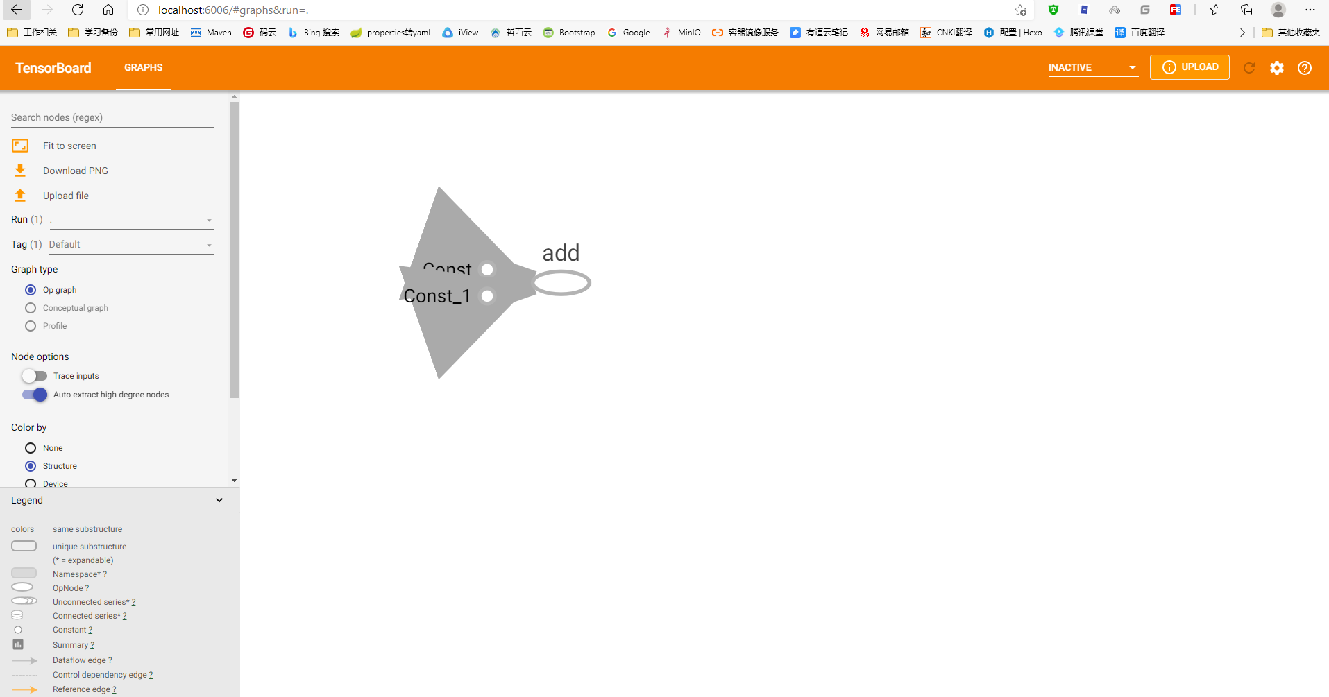
1.3.2 启动TensorBoard 启动命令如下
tensorboard --logdir="test/"
然后在浏览器中打开 http://localhost:6006/ 即可查看
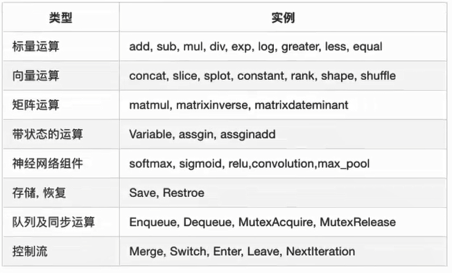
1.4 OP操作 1.4.1 基本操作 常见的OP操作
一个操作对象(Operation)是TensorFlow图中的一个节点,可以接收0个或多个输入Tensor , 并且可以输出0个或多个输入Tensor。Operation对象时通过op构造函数(如tf.matmul()) 创建的
例如 c = tf.matmul()创建了一个Operation对象,类型为Matmul类型,他将张量a,b作为输入,c作为输出,并且输出数据,打印的时候也是打印的数据。其中tf.matmul()是函数,在执行matmul()过程中会通过matmul创建一个与之对应的对象。
import tensorflow as tftf.compat.v1.disable_eager_execution() t = tf.compat.v1.compat.v1 def add () : a_t = t.constant(2 ) b_t = t.constant(3 ) c_t = t.add(a_t, b_t) print(" a_t = " , a_t, "\n" ) print(" b_t = " , b_t, "\n" ) print(" c_t = " , c_t, "\n" ) if __name__ == "__main__" : add()
运行结果为
a_t = Tensor("Const:0" , shape=(), dtype=int32) b_t = Tensor("Const_1:0" , shape=(), dtype=int32) c_t = Tensor("Add:0" , shape=(), dtype=int32)
注意打印出来的是张量值,可以理解为OP中包含了这个值,并且每一个OP指令对对应一个唯一的名称,如Const:0,这个可以在tensorboard中显示。
tf.Tensor以输出该张量的tf.Operation明确命名。张量名称的形式为”:“,其中
是生成该张量的指令的名称 是一个整数,他表示盖章量在指令的输出中的索引
1.4.2 指令名称 tf.Graph为其包含的tf.Operation对象定义的一个命名空间。TensorFlow会自动为图中的每一个指令选择一个唯一的名称,用户也可以指定描述性名称,是程序阅读起来更轻松,可以以下方式改写指令名称:
每个创建新的tf.Operation或返回的tf.Tensor的API函数可以接受可选的name参数。
import tensorflow as tftf.compat.v1.disable_eager_execution() t = tf.compat.v1.compat.v1 def add () : a_t = t.constant(2 , name="a" ) b_t = t.constant(3 , name="b" ) c_t = t.add(a_t, b_t, name="c" ) print(" a_t = " , a_t, "\n" ) print(" b_t = " , b_t, "\n" ) print(" c_t = " , c_t, "\n" ) if __name__ == "__main__" : add()
运行结果为
a_t = Tensor("a:0" , shape=(), dtype=int32) b_t = Tensor("b:0" , shape=(), dtype=int32) c_t = Tensor("c:0" , shape=(), dtype=int32)
1.5 会话 一个运行的TensorFlow Operation 的类,会话包含以下两种开启方式
tf.Session 用于完整的程序中
tf.InteractiveSession 用于交互式上下文中的TensorFlow ,例如shell
TensorFlow 使用tf.Session类表示客户端程序与C++运行时之间的连接
tf.Session对象使用分布式TensorFlow 运行时提供对本地计算机中的设备的和远程设备的访问权限
1.5.1 基本使用 会话可能拥有的资源,如 tf.Variable , tf.QueueBase 和 tf.ReaderBase ,当这些资源不需要时释放这些资源很重要,因此需要调用t.Session.close 会话中的方法或将会话用作上下文管理器。
import tensorflow as tftf.compat.v1.disable_eager_execution() t = tf.compat.v1.compat.v1 def add () : a_t = t.constant(2 , name="a" ) b_t = t.constant(3 , name="b" ) c_t = t.add(a_t, b_t, name="c" ) print(" a_t = " , a_t, "\n" ) print(" b_t = " , b_t, "\n" ) print(" c_t = " , c_t, "\n" ) with t.Session() as sess: r = sess.run([a_t, b_t, c_t]) print(" r = " , r) print("会话的图属性 = " , sess.graph) if __name__ == "__main__" : add()
运行结果为
a_t = Tensor("a:0", shape=(), dtype=int32) b_t = Tensor("b:0", shape=(), dtype=int32) c_t = Tensor("c:0", shape=(), dtype=int32) r = [2, 3, 5] 会话的图属性 = <tensorflow.python.framework.ops.Graph object at 0x0000020259F2E3A0>
而传统的开启会话的方式如下
sess = t.Session() sum_t = sess.run(c_t) print("sum_t = " , sum_t) sess.close()
这两种开启会话的方式没有区别
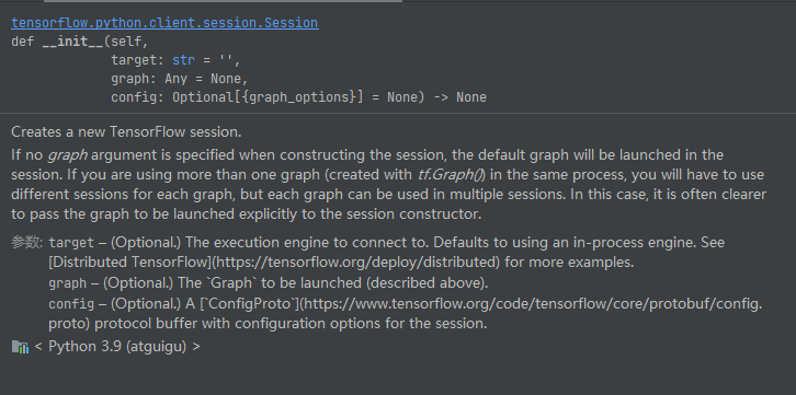
其中开启会话的接口定义如下
__init__(self, target='' , graph=None , config=None )
各参数的含义如下
graph=None
target:如果将此参数留空(默认设置),会话将仅使用本地计算机中的设备。可以指定 grpc:// 网址,以便指定 TensorFlow 服务器的地址,这使得会话可以访问该服务器控制的计算机上的所有设备。
config:此参数允许您指定一个 tf.ConfigProto 以便控制会话的行为。例如,ConfigProto协议用于打印设备使用信息
sess = t.Session(config=t.ConfigProto(allow_soft_placement=True , log_device_placement=True ))
会话可以分配不同的资源在不同的设备上运行
import tensorflow as tftf.compat.v1.disable_eager_execution() t = tf.compat.v1.compat.v1 def add () : a_t = t.constant(2 , name="a" ) b_t = t.constant(3 , name="b" ) c_t = t.add(a_t, b_t, name="c" ) print(" a_t = " , a_t, "\n" ) print(" b_t = " , b_t, "\n" ) print(" c_t = " , c_t, "\n" ) sess = t.Session(config=t.ConfigProto(allow_soft_placement=True , log_device_placement=True )) sum_t = sess.run(c_t) print("sum_t = " , sum_t) sess.close() if __name__ == "__main__" : add()
运行结果如下
 a_t  =  Tensor("a:0", shape=(), dtype=int32)
 b_t  =  Tensor("b:0", shape=(), dtype=int32)
 c_t  =  Tensor("c:0", shape=(), dtype=int32)


 2021-05-28 16:08:29.878034: I tensorflow/core/platform/cpu_feature_guard.cc:142] This TensorFlow binary is optimized with oneAPI Deep Neural Network Library (oneDNN) to use the following CPU instructions in performance-critical operations:  AVX AVX2
To enable them in other operations, rebuild TensorFlow with the appropriate compiler flags.
2021-05-28 16:08:29.932176: I tensorflow/stream_executor/platform/default/dso_loader.cc:53] Successfully opened dynamic library nvcuda.dll
2021-05-28 16:08:29.948457: E tensorflow/stream_executor/cuda/cuda_driver.cc:328] failed call to cuInit: CUDA_ERROR_UNKNOWN: unknown error
2021-05-28 16:08:29.951547: I tensorflow/stream_executor/cuda/cuda_diagnostics.cc:169] retrieving CUDA diagnostic information for host: DESKTOP-TU6LR6R
2021-05-28 16:08:29.951995: I tensorflow/stream_executor/cuda/cuda_diagnostics.cc:176] hostname: DESKTOP-TU6LR6R
2021-05-28 16:08:29.952484: I tensorflow/core/common_runtime/direct_session.cc:361] Device mapping: no known devices.

 c: (Add): /job:localhost/replica:0/task:0/device:CPU:0
 a: (Const): /job:localhost/replica:0/task:0/device:CPU:0
 b: (Const): /job:localhost/replica:0/task:0/device:CPU:0

 sum_t =  5
1.5.2 会话的run 改接口的定义如下
def run (self, fetches, feed_dict=None, options=None, run_metadata=None) :
通过sess.run( )运行operation
fetches : 单一的operation 或者列表 、元组 (其他不属于TensorFlow的类型不行)
feed_dict : 参数允许调用者覆盖图中张量的值,运行时赋值。与tf.placeholder搭配使用则会检查值的形状是否与占位符兼容
tf.operation.eval()也可以运行operation,但需要在会话中进行
对于以下代码
import tensorflow as tf2tf2.compat.v1.disable_eager_execution() tf = tf2.compat.v1.compat.v1 def add () : a = tf.constant(2.0 ) b = tf.constant(3.0 ) c = a * b sess = tf.Session() print(" sess.run(c) =" , sess.run(c)) print(" c.eval =" , c.eval(session=sess)) if __name__ == "__main__" : add()
运行结果为
sess.run(c) = 6.0
c.eval = 6.0
批量获取结果
import tensorflow as tf2tf2.compat.v1.disable_eager_execution() tf = tf2.compat.v1.compat.v1 def add () : a = tf.constant(2.0 ) b = tf.constant(3.0 ) c = a * b sess = tf.Session() s_a, s_b, s_c = sess.run((a, b, c)) print(f" 结果值为 s_a = {s_a} , s_b ={s_b} ,s_c ={s_c} " ) if __name__ == "__main__" : add()
运行结果为
结果值为 s_a = 2.0 , s_b =3.0 ,s_c =6.0
feed操作
placeholder提供占位符,run的时候通过feed_dict 指定参数
import tensorflow as tf2tf2.compat.v1.disable_eager_execution() tf = tf2.compat.v1.compat.v1 def add () : a = tf.placeholder(tf.float32) b = tf.placeholder(tf.float32) c = tf.add(a, b) print(f" f = {c} " ) with tf.Session() as sess: r = sess.run(c, feed_dict={a: 2.0 , b: 3.0 }) print(f" 结果值为 r = {r} " ) if __name__ == "__main__" : add()
运行结果为
f = Tensor("Add:0" , dtype=float32) 结果值为 r = 5.0
如果运行时报错
RuntimeError: session是无效状态,例如session已关闭
TypeError : fetches 或 feed_dict 键的类型不合适
ValueError : fetches 或 feed_dict 键无效或引用的TensorFlow不存在
示例1
import tensorflow as tf2tf2.compat.v1.disable_eager_execution() tf = tf2.compat.v1.compat.v1 def add () : a = tf.placeholder(tf.float32) b = tf.placeholder(tf.float32) c = tf.add(a, b) print(f" f = {c} " ) with tf.Session() as sess: r = sess.run(c) print(f" 结果值为 r = {r} " ) if __name__ == "__main__" : add()
结果为
f = Tensor("Add:0" , dtype=float32) 2021 -05 -28 16 :50 :11.305757 : I tensorflow/stream_executor/platform/default/dso_loader.cc:53 ] Successfully opened dynamic library nvcuda.dll2021 -05 -28 16 :50 :11.320313 : E tensorflow/stream_executor/cuda/cuda_driver.cc:328 ] failed call to cuInit: CUDA_ERROR_UNKNOWN: unknown error2021 -05 -28 16 :50 :11.323347 : I tensorflow/stream_executor/cuda/cuda_diagnostics.cc:169 ] retrieving CUDA diagnostic information for host: DESKTOP-TU6LR6R2021 -05 -28 16 :50 :11.323769 : I tensorflow/stream_executor/cuda/cuda_diagnostics.cc:176 ] hostname: DESKTOP-TU6LR6R2021 -05 -28 16 :50 :11.324418 : I tensorflow/core/platform/cpu_feature_guard.cc:142 ] This TensorFlow binary is optimized with oneAPI Deep Neural Network Library (oneDNN) to use the following CPU instructions in performance-critical operations: AVX AVX2To enable them in other operations, rebuild TensorFlow with the appropriate compiler flags. Traceback (most recent call last): File "F:\python_workspace\atguigu\venv\lib\site-packages\tensorflow\python\client\session.py" , line 1375 , in _do_call return fn(*args) File "F:\python_workspace\atguigu\venv\lib\site-packages\tensorflow\python\client\session.py" , line 1359 , in _run_fn return self._call_tf_sessionrun(options, feed_dict, fetch_list, File "F:\python_workspace\atguigu\venv\lib\site-packages\tensorflow\python\client\session.py" , line 1451 , in _call_tf_sessionrun return tf_session.TF_SessionRun_wrapper(self._session, options, feed_dict, tensorflow.python.framework.errors_impl.InvalidArgumentError: You must feed a value for placeholder tensor 'Placeholder_1' with dtype float [[{{node Placeholder_1}}]] During handling of the above exception, another exception occurred: Traceback (most recent call last): File "<input>" , line 1 , in <module> File "C:\Program Files\JetBrains\PyCharm 2021.1.1\plugins\python\helpers\pydev\_pydev_bundle\pydev_umd.py" , line 197 , in runfile pydev_imports.execfile(filename, global_vars, local_vars) File "C:\Program Files\JetBrains\PyCharm 2021.1.1\plugins\python\helpers\pydev\_pydev_imps\_pydev_execfile.py" , line 18 , in execfile exec(compile(contents+"\n" , file, 'exec' ), glob, loc) File "F:/python_workspace/atguigu/demo3.py" , line 23 , in <module> add() File "F:/python_workspace/atguigu/demo3.py" , line 18 , in add r = sess.run(c) File "F:\python_workspace\atguigu\venv\lib\site-packages\tensorflow\python\client\session.py" , line 967 , in run result = self._run(None , fetches, feed_dict, options_ptr, File "F:\python_workspace\atguigu\venv\lib\site-packages\tensorflow\python\client\session.py" , line 1190 , in _run results = self._do_run(handle, final_targets, final_fetches, File "F:\python_workspace\atguigu\venv\lib\site-packages\tensorflow\python\client\session.py" , line 1368 , in _do_run return self._do_call(_run_fn, feeds, fetches, targets, options, File "F:\python_workspace\atguigu\venv\lib\site-packages\tensorflow\python\client\session.py" , line 1394 , in _do_call raise type(e)(node_def, op, message) tensorflow.python.framework.errors_impl.InvalidArgumentError: You must feed a value for placeholder tensor 'Placeholder_1' with dtype float [[node Placeholder_1 (defined at F:/python_workspace/atguigu/demo3.py:11 ) ]] Original stack trace for 'Placeholder_1' : File "C:\Program Files\JetBrains\PyCharm 2021.1.1\plugins\python\helpers\pydev\pydevconsole.py" , line 483 , in <module> pydevconsole.start_client(host, port) File "C:\Program Files\JetBrains\PyCharm 2021.1.1\plugins\python\helpers\pydev\pydevconsole.py" , line 411 , in start_client process_exec_queue(interpreter) File "C:\Program Files\JetBrains\PyCharm 2021.1.1\plugins\python\helpers\pydev\pydevconsole.py" , line 258 , in process_exec_queue interpreter.add_exec(code_fragment) File "C:\Program Files\JetBrains\PyCharm 2021.1.1\plugins\python\helpers\pydev\_pydev_bundle\pydev_code_executor.py" , line 106 , in add_exec more = self.do_add_exec(code_fragment) File "C:\Program Files\JetBrains\PyCharm 2021.1.1\plugins\python\helpers\pydev\pydevconsole.py" , line 84 , in do_add_exec command.run() File "C:\Program Files\JetBrains\PyCharm 2021.1.1\plugins\python\helpers\pydev\_pydev_bundle\pydev_console_types.py" , line 35 , in run self.more = self.interpreter.runsource(text, '<input>' , symbol) File "C:\Users\yishui\AppData\Local\Programs\Python\Python39\lib\code.py" , line 74 , in runsource self.runcode(code) File "C:\Users\yishui\AppData\Local\Programs\Python\Python39\lib\code.py" , line 90 , in runcode exec(code, self.locals) File "<input>" , line 1 , in <module> File "C:\Program Files\JetBrains\PyCharm 2021.1.1\plugins\python\helpers\pydev\_pydev_bundle\pydev_umd.py" , line 197 , in runfile pydev_imports.execfile(filename, global_vars, local_vars) File "C:\Program Files\JetBrains\PyCharm 2021.1.1\plugins\python\helpers\pydev\_pydev_imps\_pydev_execfile.py" , line 18 , in execfile exec(compile(contents+"\n" , file, 'exec' ), glob, loc) File "F:/python_workspace/atguigu/demo3.py" , line 23 , in <module> add() File "F:/python_workspace/atguigu/demo3.py" , line 11 , in add b = tf.placeholder(tf.float32) File "F:\python_workspace\atguigu\venv\lib\site-packages\tensorflow\python\ops\array_ops.py" , line 3271 , in placeholder return gen_array_ops.placeholder(dtype=dtype, shape=shape, name=name) File "F:\python_workspace\atguigu\venv\lib\site-packages\tensorflow\python\ops\gen_array_ops.py" , line 6744 , in placeholder _, _, _op, _outputs = _op_def_library._apply_op_helper( File "F:\python_workspace\atguigu\venv\lib\site-packages\tensorflow\python\framework\op_def_library.py" , line 748 , in _apply_op_helper op = g._create_op_internal(op_type_name, inputs, dtypes=None , File "F:\python_workspace\atguigu\venv\lib\site-packages\tensorflow\python\framework\ops.py" , line 3557 , in _create_op_internal ret = Operation( File "F:\python_workspace\atguigu\venv\lib\site-packages\tensorflow\python\framework\ops.py" , line 2045 , in __init__ self._traceback = tf_stack.extract_stack_for_node(self._c_op)
示例2
import tensorflow as tf2tf2.compat.v1.disable_eager_execution() tf = tf2.compat.v1.compat.v1 def add () : a = tf.placeholder(tf.float32) b = tf.placeholder(tf.float32) c = tf.add(a, b) print(f" f = {c} " ) with tf.Session() as sess: r = sess.run(c, feed_dict={a: "asas" , b: 3.0 }) print(f" 结果值为 r = {r} " ) if __name__ == "__main__" : add()
运行结果为
2021 -05 -28 16 :53 :40.909120 : W tensorflow/stream_executor/platform/default/dso_loader.cc:64 ] Could not load dynamic library 'cudart64_110.dll' ; dlerror: cudart64_110.dll not found2021 -05 -28 16 :53 :40.909472 : I tensorflow/stream_executor/cuda/cudart_stub.cc:29 ] Ignore above cudart dlerror if you do not have a GPU set up on your machine. f = Tensor("Add:0" , dtype=float32) 2021 -05 -28 16 :53 :44.855138 : I tensorflow/stream_executor/platform/default/dso_loader.cc:53 ] Successfully opened dynamic library nvcuda.dll2021 -05 -28 16 :53 :44.868947 : E tensorflow/stream_executor/cuda/cuda_driver.cc:328 ] failed call to cuInit: CUDA_ERROR_UNKNOWN: unknown error2021 -05 -28 16 :53 :44.871899 : I tensorflow/stream_executor/cuda/cuda_diagnostics.cc:169 ] retrieving CUDA diagnostic information for host: DESKTOP-TU6LR6R2021 -05 -28 16 :53 :44.872321 : I tensorflow/stream_executor/cuda/cuda_diagnostics.cc:176 ] hostname: DESKTOP-TU6LR6R2021 -05 -28 16 :53 :44.872955 : I tensorflow/core/platform/cpu_feature_guard.cc:142 ] This TensorFlow binary is optimized with oneAPI Deep Neural Network Library (oneDNN) to use the following CPU instructions in performance-critical operations: AVX AVX2To enable them in other operations, rebuild TensorFlow with the appropriate compiler flags. Traceback (most recent call last): File "<input>" , line 1 , in <module> File "C:\Program Files\JetBrains\PyCharm 2021.1.1\plugins\python\helpers\pydev\_pydev_bundle\pydev_umd.py" , line 197 , in runfile pydev_imports.execfile(filename, global_vars, local_vars) File "C:\Program Files\JetBrains\PyCharm 2021.1.1\plugins\python\helpers\pydev\_pydev_imps\_pydev_execfile.py" , line 18 , in execfile exec(compile(contents+"\n" , file, 'exec' ), glob, loc) File "F:/python_workspace/atguigu/demo3.py" , line 23 , in <module> add() File "F:/python_workspace/atguigu/demo3.py" , line 17 , in add r = sess.run(c, feed_dict={a: "asas" , b: 3.0 }) File "F:\python_workspace\atguigu\venv\lib\site-packages\tensorflow\python\client\session.py" , line 967 , in run result = self._run(None , fetches, feed_dict, options_ptr, File "F:\python_workspace\atguigu\venv\lib\site-packages\tensorflow\python\client\session.py" , line 1160 , in _run np_val = np.asarray(subfeed_val, dtype=subfeed_dtype) File "F:\python_workspace\atguigu\venv\lib\site-packages\numpy\core\_asarray.py" , line 83 , in asarray return array(a, dtype, copy=False , order=order) ValueError: could not convert string to float: 'asas'
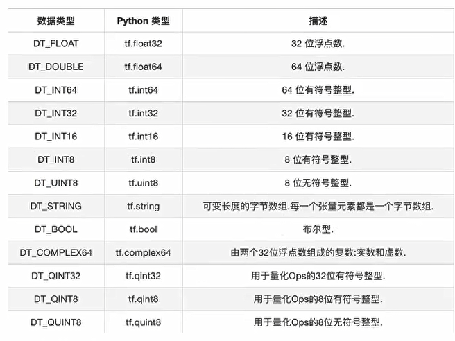
1.6 张量 在编写TensorFlow程序时,程序传递和运算的主要目标是tf.Tensor
TensorFlow的张量就是一个N维数组,类型为tf.Tensor。Tensor具有以下两个重要属性
TensorFlow 支持以下三种类型的张量:
常量:常量是其值不能改变的张量。
变量:当一个量在会话中的值需要更新时,使用变量来表示。例如,在神经网络中,权重需要在训练期间更新,可以通过将权重声明为变量来实现。变量在使用前需要被显示初始化。另外需要注意的是,常量存储在计算图的定义中,每次加载图时都会加载相关变量。换句话说,它们是占用内存的。另一方面,变量又是分开存储的。它们可以存储在参数服务器上。
占位符:用于将值输入 TensorFlow 图中。它们可以和 feed_dict 一起使用来输入数据。在训练神经网络时,它们通常用于提供新的训练样本。在会话中运行计算图时,可以为占位符赋值。这样在构建一个计算图时不需要真正地输入数据。需要注意的是,占位符不包含任何数据,因此不需要初始化它们。
张量的类型
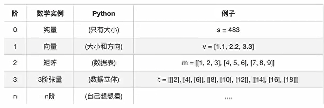
张量的阶
示例如下
tensor1 = tf.constant(4.0 ) tensor2 = tf.constant([1 , 2 , 3 , 4 ]) linear_squares = tf.constant([[4 ], [9 ], [16 ], [25 ]], dtype=tf.int32)
1.6.1 属性与生成 1.6.1.1 TensorFlow 常量
声明一个标量常量:
一个形如 [1,3] 的常量向量可以用如下代码声明:
t_2 = tf.constant([4 ,3 ,2 ])
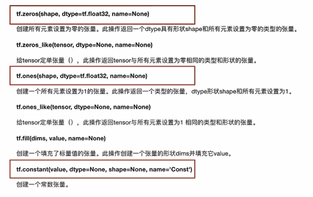
要创建一个所有元素为零的张量,可以使用 tf.zeros() 函数。这个语句可以创建一个形如 [M,N] 的零元素矩阵,数据类型(dtype)可以是 int32、float32 等:
例如:
zero_t = tf.zeros([2 ,3 ],tf.int32)
还可以创建与现有 Numpy 数组或张量常量具有相同形状的张量常量,如下所示:
创建一个所有元素都设为 1 的张量。下面的语句即创建一个形如 [M,N]、元素均为 1 的矩阵:
例如:
ones_t = tf.ones([2 ,3 ],tf.int32)
在一定范围内生成一个从初值到终值等差排布的序列:
tf.linspace(start,stop,num)
相应的值为 (stop-start)/(num-1)。例如:
range_t = tf.linspace(2.0 ,5.0 ,5 )
从开始(默认值=0)生成一个数字序列,增量为 delta(默认值=1),直到终值(但不包括终值):
tf.range(start,limit,delta)
实例:
TensorFlow 允许创建具有不同分布的随机张量:
1 : 使用以下语句创建一个具有一定均值(默认值=0.0)和标准差(默认值=1.0)、形状为 [M,N] 的正态分布随机数组 :
import tensorflow as tf2tf2.compat.v1.disable_eager_execution() tf = tf2.compat.v1.compat.v1 def demo () : val = tf.random_normal([2 , 3 ], mean=2.0 , stddev=4 , seed=12 ) print(val) with tf.Session() as sess: print(sess.run(val)) if __name__ == "__main__" : demo()
输出结果为
Tensor("random_normal:0" , shape=(2 , 3 ), dtype=float32) [[ 0.25347447 5.37991 1.9527606 ] [-1.5376031 1.2588985 2.8478067 ]]
2 :创建一个具有一定均值(默认值=0.0)和标准差(默认值=1.0)、形状为 [M,N] 的截尾正态分布随机数组
import tensorflow as tf2tf2.compat.v1.disable_eager_execution() tf = tf2.compat.v1.compat.v1 def demo () : val = tf.truncated_normal([1 , 5 ], stddev=2 , seed=12 ) print(val) with tf.Session() as sess: print(sess.run(val)) if __name__ == "__main__" : demo()
运行结果为
Tensor("truncated_normal:0" , shape=(1 , 5 ), dtype=float32) [[-0.87326276 1.689955 -0.02361972 -1.7688016 -3.87749 ]]
3 : 要在种子的 [minval(default=0),maxval] 范围内创建形状为 [M,N] 的给定伽马分布随机数组 ,请执行如下语句:
import tensorflow as tf2tf2.compat.v1.disable_eager_execution() tf = tf2.compat.v1.compat.v1 def demo () : val = tf.random_uniform([2 , 3 ], maxval=4 , seed=12 ) print(val) with tf.Session() as sess: print(sess.run(val)) if __name__ == "__main__" : demo()
输出结果为
Tensor("random_uniform/Mul:0" , shape=(2 , 3 ), dtype=float32) [[2.54461 3.6963658 2.7051091 ] [2.0085006 3.8445983 3.5426888 ]]
要将给定的张量随机裁剪为指定的大小,使用以下语句:
tf.random_crop(t_random,[2 ,5 ],seed=12 )
这里,t_random 是一个已经定义好的张量。这将导致随机从张量 t_random 中裁剪出一个大小为 [2,5] 的张量。
很多时候需要以随机的顺序来呈现训练样本,可以使用 tf.random_shuffle() 来沿着它的第一维随机排列张量。如果 t_random 是想要重新排序的张量,使用下面的代码:
tf.random_shuffle(t_random)
随机生成的张量受初始种子值的影响。要在多次运行或会话中获得相同的随机数,应该将种子设置为一个常数值。当使用大量的随机张量时,可以使用 tf.set_random_seed() 来为所有随机产生的张量设置种子。以下命令将所有会话的随机张量的种子设置为 54:
种子只能有整数值。
1.6.1.2 TensorFlow 变量 TensorFlow变量是表示程序处理的共享持久状态的最佳方法,变量通过OP类进行操作,变量的特点为
它们通过使用变量类来创建。变量的定义还包括应该初始化的常量/随机值。下面的代码中创建了两个不同的张量变量 t_a 和 t_b。两者将被初始化为形状为 [50,50] 的随机均匀分布,最小值=0,最大值=10:
ran_val = tf.random_uniform([50 , 50 ], 0 , 10 , seed=12 ) var_a = tf.Variable(ran_val) var_b = tf.Variable(ran_val) print(f" ran_val = {ran_val} \n" ) print(f" var_a = {var_a} \n" ) print(f" var_b = {var_b} \n" )
运行结果为
ran_val = Tensor("random_uniform/Mul:0" , shape=(50 , 50 ), dtype=float32) var_a = <tf.Variable 'Variable:0' shape=(50 , 50 ) dtype=float32> var_b = <tf.Variable 'Variable_1:0' shape=(50 , 50 ) dtype=float32>
注意:变量通常在神经网络中表示权重和偏置。
下面的代码中定义了两个变量的权重和偏置。权重变量使用正态分布随机初始化,均值为 0,标准差为 2,权重大小为 100×100。偏置由 100 个元素组成,每个元素初始化为 0。在这里也使用了可选参数名以给计算图中定义的变量命名:
在前面的例子中,都是利用一些常量来初始化变量,也可以指定一个变量来初始化另一个变量。下面的语句将利用前面定义的权重来初始化 weight2:
变量的定义将指定变量如何被初始化,但是必须显式初始化所有的声明变量。在计算图的定义中通过声明初始化操作对象来实现:
每个变量也可以在运行图中单独使用 tf.Variable.initializer 来初始化:
import tensorflow as tf2tf2.compat.v1.disable_eager_execution() tf = tf2.compat.v1.compat.v1 def demo () : ran_val = tf.random_uniform([50 , 50 ], 0 , 10 , seed=12 ) var_a = tf.Variable(ran_val) var_b = tf.Variable(ran_val) print(f" ran_val = {ran_val} \n" ) print(f" var_a = {var_a} \n" ) print(f" var_b = {var_b} \n" ) init = tf.global_variables_initializer() with tf.Session() as sess: sess.run(init) t_ran_val, t_var_a, t_var_b = sess.run([ran_val, var_a, var_b]) print(f" ran_val 的实际值为 = {t_ran_val} \n" ) print(f" var_a 的实际值为 = {t_var_a} \n" ) print(f" var_b 的实际值为 = {t_var_b} \n" ) if __name__ == "__main__" : demo()
运行结果为
ran_val 的实际值为 = [[7.4577665 8.163866 0.84701896 ... 4.1017447 4.7203207 0.5532837 ] [0.20663738 7.7947006 9.814263 ... 8.367065 6.777916 2.6292324 ] [6.4287186 0.04263043 2.9992056 ... 3.4029925 3.4579408 6.335558 ] ... [6.0129585 0.3255713 7.652465 ... 6.0094223 8.154499 0.6161797 ] [7.709612 0.08945107 8.787935 ... 8.848581 6.1873436 3.5578668 ] [2.3331022 2.7387297 5.2715683 ... 9.044791 9.005299 6.6066084 ]] var_a 的实际值为 = [[6.361525 9.240914 6.7627726 ... 6.6943073 6.7619324 8.1915865 ] [2.3830903 7.821268 3.8752866 ... 3.0914688 9.821395 6.052549 ] [8.715414 0.3154695 7.130703 ... 9.408816 3.2833254 3.0787969 ] ... [1.3317215 2.5219142 7.073233 ... 3.5557294 6.748437 1.8760192 ] [4.60027 7.792387 9.947163 ... 4.2264547 9.478819 5.579261 ] [7.1508207 6.8793592 2.9773557 ... 1.0567057 9.911671 3.3584273 ]] var_b 的实际值为 = [[6.361525 9.240914 6.7627726 ... 6.6943073 6.7619324 8.1915865 ] [2.3830903 7.821268 3.8752866 ... 3.0914688 9.821395 6.052549 ] [8.715414 0.3154695 7.130703 ... 9.408816 3.2833254 3.0787969 ] ... [1.3317215 2.5219142 7.073233 ... 3.5557294 6.748437 1.8760192 ] [4.60027 7.792387 9.947163 ... 4.2264547 9.478819 5.579261 ] [7.1508207 6.8793592 2.9773557 ... 1.0567057 9.911671 3.3584273 ]]
必须执行变量初始化操作,否则在获取实际值的步骤时会出现问题!!!!!
tensorflow.python.framework.errors_impl.FailedPreconditionError: Could not find variable Variable. This could mean that the variable has been deleted. In TF1, it can also mean the variable is uninitialized. Debug info: container=localhost, status=Not found: Container localhost does not exist. (Could not find resource: localhost/Variable) [[node Variable/Read/ReadVariableOp (defined at F:/python_workspace/atguigu/demo6.py:10 ) ]]
修改变量的命名空间
import tensorflow as tf2tf2.compat.v1.disable_eager_execution() tf = tf2.compat.v1.compat.v1 def demo () : with tf.variable_scope("my_scop" ): var_a = tf.Variable(initial_value=50 ) var_b = tf.Variable(initial_value=50 ) print(f" var_a = {var_a} \n" ) print(f" var_b = {var_b} \n" ) init = tf.global_variables_initializer() with tf.Session() as sess: sess.run(init) t_var_a, t_var_b = sess.run([var_a, var_b]) print(f" var_a 的实际值为 = {t_var_a} \n" ) print(f" var_b 的实际值为 = {t_var_b} \n" ) if __name__ == "__main__" : demo()
运行结果为
var_a = <tf.Variable 'my_scop/Variable:0' shape=() dtype=int32>
var_b = <tf.Variable 'my_scop/Variable_1:0' shape=() dtype=int32>

 var_a 的实际值为 = 50
var_b 的实际值为 = 50
保存变量:使用 Saver 类来保存变量,定义一个 Saver 操作对象:
1.6.1.3 TensorFlow 占位符 介绍完常量和变量之后,我们来讲解最重要的元素——占位符,它们用于将数据提供给计算图。可以使用以下方法定义一个占位符:
tf.placeholder(dtype,shape=None ,name=None )
dtype 定占位符的数据类型,并且必须在声明占位符时指定。在这里,为 x 定义一个占位符并计算 y=2*x,使用 feed_dict 输入一个随机的 4×5 矩阵:
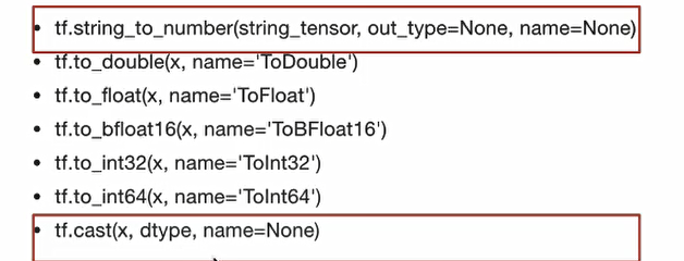
1.6.2 张量的改变 类型的改变
形状的改变
TensorFlow的张量具有两种形状变换,动态形状和静态形状
静态形状 - 初始创建张量时的形状
2)如何改变动态形状
不会改变原始的tensor
tf.reshape(tensor, shape)
2)如何改变动态形状
关于静态形状和动态形状必须符合一下规则
静态形状
转换静态形状时,1-D到D-1,2-D到D-2不能跨阶数改变(即必须一维到一维,二维到二维,不能跨阶数改变)
对于已经固定的张量的静态形状的张量,不能再次设置静态形状
动态形状
tf.reshape()动态创建新张量时,张量的元素个数必须匹配
import tensorflow as tf2tf2.compat.v1.disable_eager_execution() tf = tf2.compat.v1.compat.v1 def demo () : """ 张量的演示 :return: """ tensor1 = tf.constant(4.0 ) tensor2 = tf.constant([1 , 2 , 3 , 4 ]) linear_squares = tf.constant([[4 ], [9 ], [16 ], [25 ]], dtype=tf.int32) print(f"tensor1:{tensor1} \n" ) print(f"tensor2:{tensor2} \n" ) print(f"linear_squares_before:{linear_squares} \n" ) l_cast = tf.cast(linear_squares, dtype=tf.float32) print(f"linear_squares_after:{linear_squares} \n" ) print(f"l_cast:{l_cast} \n" ) a_p = tf.placeholder(dtype=tf.float32, shape=[None , None ]) b_p = tf.placeholder(dtype=tf.float32, shape=[None , 10 ]) c_p = tf.placeholder(dtype=tf.float32, shape=[3 , 2 ]) print("=============== 没有完全固定下来的静态形状 ===================" ) print(f"固定前 a_p: {a_p} \n" ) print(f"固定前 b_p:{b_p} \n" ) print(f"固定前 c_p:{c_p} \n" ) a_p.set_shape([2 , 3 ]) b_p.set_shape([2 , 10 ]) print("=============== 更新形状未确定的部分 ===================" ) print(f"更新后 a_p: {a_p} \n" ) print(f"更新后 b_p:{b_p} \n" ) a_p_reshape = tf.reshape(a_p, shape=[2 , 3 , 1 ]) print("=============== 动态形状修改 ===================" ) print(f"a_p:{a_p} \n" ) print(f"a_p_reshape:{a_p_reshape} \n" ) print("=============== 再次动态形状修改 ===================" ) c_p_reshape = tf.reshape(c_p, shape=[2 , 3 ]) print(f"c_p:{c_p} \n" ) print(f"c_p_reshape:{c_p_reshape} \n" ) if __name__ == "__main__" : demo()
运行结果为
tensor1:Tensor("Const:0" , shape=(), dtype=float32) tensor2:Tensor("Const_1:0" , shape=(4 ,), dtype=int32) linear_squares_before:Tensor("Const_2:0" , shape=(4 , 1 ), dtype=int32) linear_squares_after:Tensor("Const_2:0" , shape=(4 , 1 ), dtype=int32) l_cast:Tensor("Cast:0" , shape=(4 , 1 ), dtype=float32) =============== 没有完全固定下来的静态形状 =================== 固定前 a_p: Tensor("Placeholder:0" , shape=(None , None ), dtype=float32) 固定前 b_p:Tensor("Placeholder_1:0" , shape=(None , 10 ), dtype=float32) 固定前 c_p:Tensor("Placeholder_2:0" , shape=(3 , 2 ), dtype=float32) =============== 更新形状未确定的部分 =================== 更新后 a_p: Tensor("Placeholder:0" , shape=(2 , 3 ), dtype=float32) 更新后 b_p:Tensor("Placeholder_1:0" , shape=(2 , 10 ), dtype=float32) =============== 动态形状修改 =================== a_p:Tensor("Placeholder:0" , shape=(2 , 3 ), dtype=float32) a_p_reshape:Tensor("Reshape:0" , shape=(2 , 3 , 1 ), dtype=float32) =============== 再次动态形状修改 =================== c_p:Tensor("Placeholder_2:0" , shape=(3 , 2 ), dtype=float32) c_p_reshape:Tensor("Reshape_1:0" , shape=(2 , 3 ), dtype=float32) import sys; print('Python %s on %s' % (sys.version, sys.platform))
1.6.3 张量的运算 具体的API的使用方法参考
Module: tf.math | TensorFlow Core v2.5.0 (google.cn)
TensorFlow 函数介绍_w3cschool
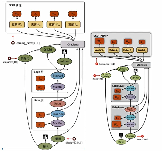
1.7 案例:TensorFlow实现线性回归 1.7.1 基础入门 构建线性回归的步骤如下
   1)构建模型
        y = w1x1 + w2x2 + …… + wnxn + b
    2)构造损失函数
        均方误差
    3)优化损失
        梯度下降
下面模拟一个线性回归的场景,其步骤如下
1  准备真实数据
   100样本
    x 特征值 形状 (100, 1)
    y_true 目标值 (100, 1)
    y_true = 0.8x + 0.7

2   假定x 和 y 之间的关系 满足
    y = kx + b
     k ≈ 0.8 b ≈ 0.7


流程分析:
     (100, 1) * (1, 1) = (100, 1)
    y_predict = x * weights(1, 1) + bias(1, 1)

1)构建模型
# matmul矩阵乘法
y_predict = tf.matmul(x, weights) + bias

2)构造损失函数
# 这里是预测值与真实值的均方误差
error = tf.reduce_mean(tf.square(y_predict - y_true))

3)优化损失
# 这里使用的梯度下降优化器
optimizer = tf.train.GradientDescentOptimizer(learning_rate=0.01).minimize(error)
代码如下
import tensorflow as tf2tf2.compat.v1.disable_eager_execution() tf = tf2.compat.v1.compat.v1 def demo () : """ 自实现一个线性回归 y = 0.8x+0.7 :return: """ X = tf.random_normal(shape=[100 , 1 ], name="feature" ) y_true = tf.matmul(X, [[0.8 ]]) + 0.7 weights = tf.Variable(initial_value=tf.random_normal(shape=[1 , 1 ]), name="Weights" ) bias = tf.Variable(initial_value=tf.random_normal(shape=[1 , 1 ]), name="Bias" ) y_predict = tf.matmul(X, weights) + bias error = tf.reduce_mean(tf.square(y_predict - y_true)) optimizer = tf.train.GradientDescentOptimizer(learning_rate=0.01 ).minimize(error) init = tf.global_variables_initializer() with tf.Session() as sess: sess.run(init) print("训练前模型参数为:权重%f,偏置%f,损失为%f" % (weights.eval(), bias.eval(), error.eval())) for i in range(1000 ): sess.run(optimizer) print("第%d次训练后模型参数为:权重%f,偏置%f,损失为%f" % (i + 1 , weights.eval(), bias.eval(), error.eval())) print("训练后模型参数为:权重%f,偏置%f,损失为%f" % (weights.eval(), bias.eval(), error.eval())) if __name__ == "__main__" : demo()
运行结果为
训练前模型参数为:权重0.330986,偏置-1.441732,损失为4.837440
第1次训练后模型参数为:权重0.333085,偏置-1.400813,损失为4.748821
第2次训练后模型参数为:权重0.348015,偏置-1.357541,损失为4.641252
第3次训练后模型参数为:权重0.352640,偏置-1.317162,损失为4.566151
..........
第999次训练后模型参数为:权重0.799999,偏置0.699999,损失为0.000000
第1000次训练后模型参数为:权重0.799999,偏置0.699999,损失为0.000000
训练后模型参数为:权重0.799999,偏置0.699999,损失为0.000000
学习率越大,训练到较好结果的步数就越少,学习率越小,训练到较好结果的步数就越大。
学习率过大会出现梯度爆炸的现象(在极端情况下,权重的值变得非常大,以至于溢出,导致出现NaN值)
出现梯度爆炸时,一般解决办法如下
重新设计网络
调准学习率
使用梯度截断(在训练过程中检查和限制梯度的大小)
使用激活函数
梯度爆炸示例
import tensorflow as tf2tf2.compat.v1.disable_eager_execution() tf = tf2.compat.v1.compat.v1 def demo () : """ 自实现一个线性回归 y = 0.8x+0.7 :return: """ X = tf.random_normal(shape=[100 , 1 ], name="feature" ) y_true = tf.matmul(X, [[0.8 ]]) + 0.7 weights = tf.Variable(initial_value=tf.random_normal(shape=[1 , 1 ]), name="Weights" ) bias = tf.Variable(initial_value=tf.random_normal(shape=[1 , 1 ]), name="Bias" ) y_predict = tf.matmul(X, weights) + bias error = tf.reduce_mean(tf.square(y_predict - y_true)) optimizer = tf.train.GradientDescentOptimizer(learning_rate=1.5 ).minimize(error) init = tf.global_variables_initializer() with tf.Session() as sess: sess.run(init) print("训练前模型参数为:权重%f,偏置%f,损失为%f" % (weights.eval(), bias.eval(), error.eval())) for i in range(1000 ): sess.run(optimizer) print("第%d次训练后模型参数为:权重%f,偏置%f,损失为%f" % (i + 1 , weights.eval(), bias.eval(), error.eval())) print("训练后模型参数为:权重%f,偏置%f,损失为%f" % (weights.eval(), bias.eval(), error.eval())) if __name__ == "__main__" : demo()
结果如下
训练前模型参数为:权重0.199251,偏置-0.445173,损失为1.742285
第1次训练后模型参数为:权重1.770046,偏置3.006634,损失为6.885912
第2次训练后模型参数为:权重-1.272060,偏置-3.705992,损失为24.729263
第3次训练后模型参数为:权重5.941316,偏置10.325886,损失为112.113945
第4次训练后模型参数为:权重-2.205094,偏置-16.134655,损失为299.354523
......
第996次训练后模型参数为:权重nan,偏置nan,损失为nan
第997次训练后模型参数为:权重nan,偏置nan,损失为nan
第998次训练后模型参数为:权重nan,偏置nan,损失为nan
第999次训练后模型参数为:权重nan,偏置nan,损失为nan
第1000次训练后模型参数为:权重nan,偏置nan,损失为nan
训练后模型参数为:权重nan,偏置nan,损失为nan
注意,这里权重是在变化的,若权重设置为不可以彼岸
weights = tf.Variable(initial_value=tf.random_normal(shape=[1 , 1 ]), trainable=False , name="Weights" )
则得到的结果为
训练前模型参数为:权重-0.435779,偏置0.493763,损失为1.693405
第1次训练后模型参数为:权重-0.435779,偏置1.165136,损失为1.978969
第2次训练后模型参数为:权重-0.435779,偏置0.010009,损失为1.996013
第3次训练后模型参数为:权重-0.435779,偏置1.863203,损失为2.964688
第4次训练后模型参数为:权重-0.435779,偏置-1.979727,损失为7.979872
第5次训练后模型参数为:权重-0.435779,偏置5.558542,损失为26.453764
1.7.2 增加变量显示
创建事件文件
收集变量
合并变量
每次迭代运行一次合并变量
每次迭代将summary对象写入事件文件
目的是在tensorBoard中观察模型的参数、损失值等变量值的变化
1 收集变量
tf.summary.scalar(name=””, tensor) 收集对于损失函数和准确率等单值变量,name为变量名字,tensor为值
tf.summary.histogram(name=””, tensor) 收集高纬度的变量参数
tf.summary.image(name=””, tensor) 收集输入的图片的张量能显示图片
2 合并变量写入事件
merged = tf.summary.merge_all()
运行合并 summary = sess.run(merged) ,每次迭代都需运行
添加 file_writer.add_summary(summary, i),i表示是第几次的值
示例如下
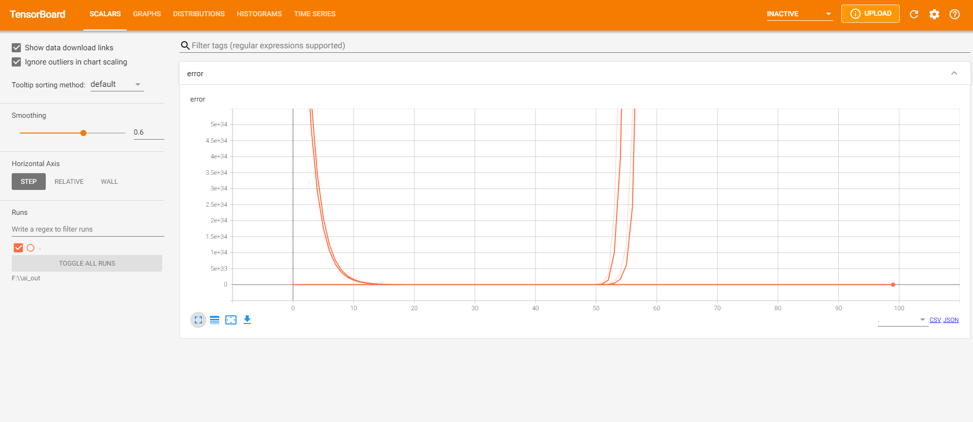
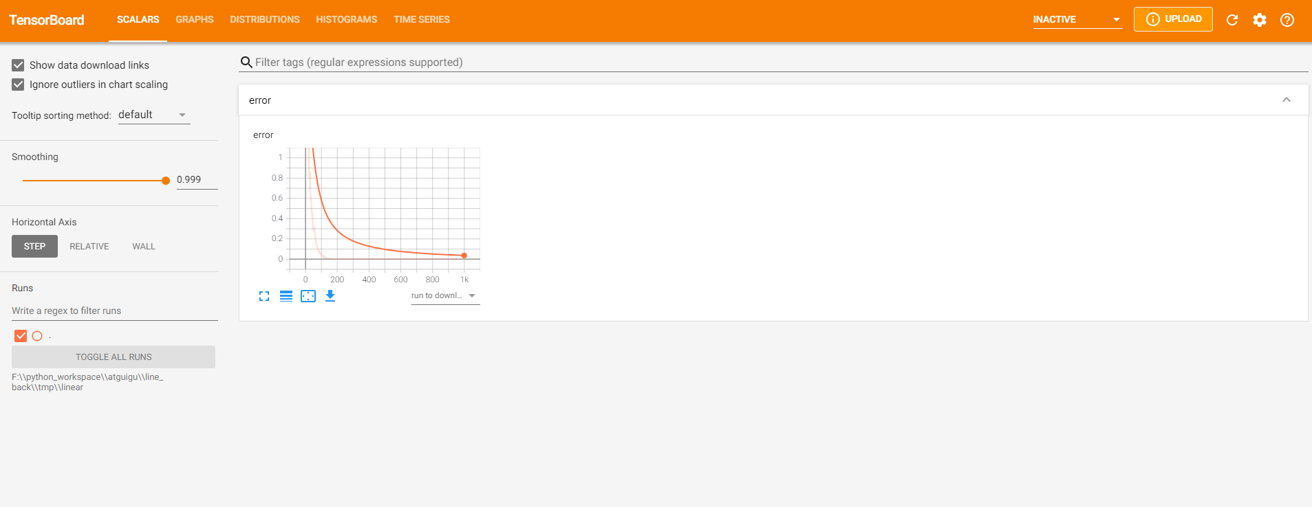
import tensorflow as tf2tf2.compat.v1.disable_eager_execution() tf = tf2.compat.v1.compat.v1 def demo () : """ 自实现一个线性回归 y = 0.8x+0.7 :return: """ X = tf.random_normal(shape=[100 , 1 ], name="feature" ) y_true = tf.matmul(X, [[0.8 ]]) + 0.7 weights = tf.Variable(initial_value=tf.random_normal(shape=[1 , 1 ]), name="Weights" ) bias = tf.Variable(initial_value=tf.random_normal(shape=[1 , 1 ]), name="Bias" ) y_predict = tf.matmul(X, weights) + bias error = tf.reduce_mean(tf.square(y_predict - y_true)) optimizer = tf.train.GradientDescentOptimizer(learning_rate=0.2 ).minimize(error) tf.summary.scalar("error" , error) tf.summary.histogram("Weights" , weights) tf.summary.histogram("Bias" , bias) merge = tf.summary.merge_all() init = tf.global_variables_initializer() with tf.Session() as sess: sess.run(init) fileWrite = tf.summary.FileWriter("F:\\ai_out" , graph=sess.graph) print("训练前模型参数为:权重%f,偏置%f,损失为%f" % (weights.eval(), bias.eval(), error.eval())) for i in range(100 ): sess.run(optimizer) summary = sess.run(merge) fileWrite.add_summary(summary, i) print("第%d次训练后模型参数为:权重%f,偏置%f,损失为%f" % (i + 1 , weights.eval(), bias.eval(), error.eval())) print("训练后模型参数为:权重%f,偏置%f,损失为%f" % (weights.eval(), bias.eval(), error.eval())) if __name__ == "__main__" : demo()
接下来运行
tensorboard --logdir="F:\\ai_out"
访问 TensorBoard (http://localhost:6006/#scalars) 可以看到
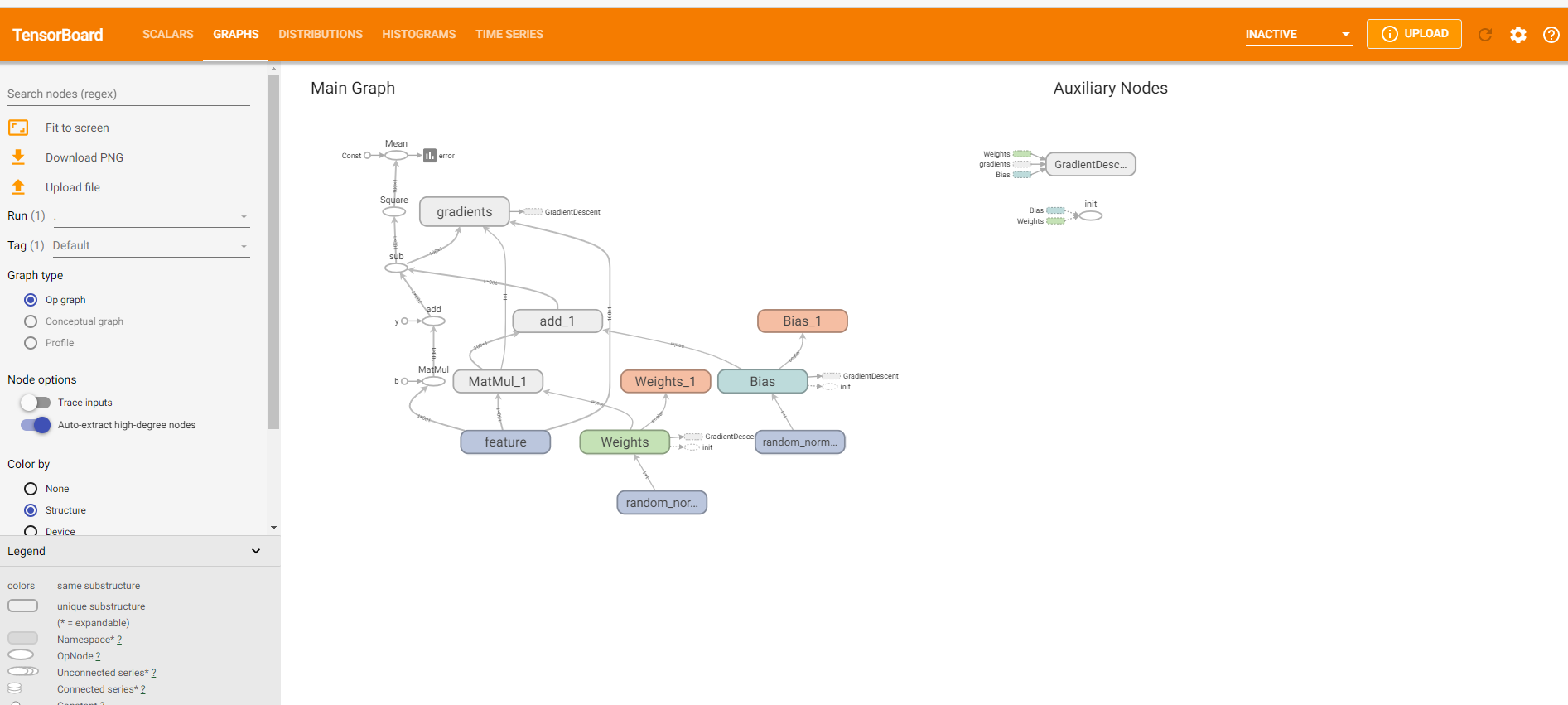
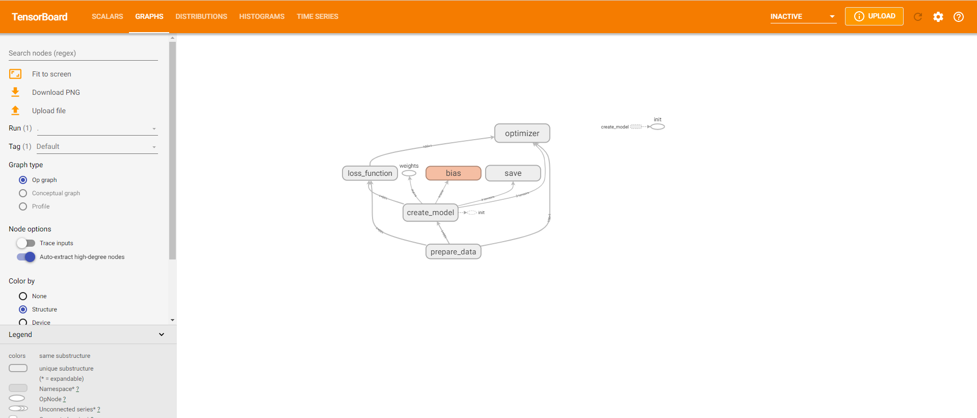
1.7.3 增加命名空间 示例代码如下
import osimport tensorflow as tf2tf2.compat.v1.disable_eager_execution() tf = tf2.compat.v1.compat.v1 def demo () : """ 自实现一个线性回归 y = 0.8x+0.7 :return: """ with tf.variable_scope("prepare_data" ): X = tf.random_normal(shape=[100 , 1 ], name="feature" ) y_true = tf.matmul(X, [[0.8 ]]) + 0.7 with tf.variable_scope("create_model" ): weights = tf.Variable(initial_value=tf.random_normal(shape=[1 , 1 ]), name="Weights" ) bias = tf.Variable(initial_value=tf.random_normal(shape=[1 , 1 ]), name="Bias" ) y_predict = tf.matmul(X, weights) + bias with tf.variable_scope("loss_function" ): error = tf.reduce_mean(tf.square(y_predict - y_true)) with tf.variable_scope("optimizer" ): optimizer = tf.train.GradientDescentOptimizer(learning_rate=0.01 ).minimize(error) tf.summary.scalar("error" , error) tf.summary.histogram("weights" , weights) tf.summary.histogram("bias" , bias) merged = tf.summary.merge_all() init = tf.global_variables_initializer() with tf.Session() as sess: sess.run(init) file_writer = tf.summary.FileWriter("./tmp/linear" , graph=sess.graph) print("训练前模型参数为:权重%f,偏置%f,损失为%f" % (weights.eval(), bias.eval(), error.eval())) for i in range(1000 ): sess.run(optimizer) print("第%d次训练后模型参数为:权重%f,偏置%f,损失为%f" % (i + 1 , weights.eval(), bias.eval(), error.eval())) summary = sess.run(merged) file_writer.add_summary(summary, i) print("训练后模型参数为:权重%f,偏置%f,损失为%f" % (weights.eval(), bias.eval(), error.eval())) if __name__ == "__main__" : demo()
结果为
训练前模型参数为:权重-1.202373,偏置-0.332873,损失为5.143828
第1次训练后模型参数为:权重-1.161383,偏置-0.311727,损失为6.317729
第2次训练后模型参数为:权重-1.106612,偏置-0.292419,损失为4.150044
第3次训练后模型参数为:权重-1.070605,偏置-0.273911,损失为4.797676
.........
第999次训练后模型参数为:权重0.799999,偏置0.699999,损失为0.000000
第1000次训练后模型参数为:权重0.799999,偏置0.699999,损失为0.000000
训练后模型参数为:权重0.799999,偏置0.699999,损失为0.000000
运行
tensorboard --logdir="F:\\python_workspace\\atguigu\\line_back\\tmp\\linear"
得到如下结果
1.7.4 模型的保存与加载 保存模型
tf.train.Saver(var_list=None,max_to_keep=5)
保存和加载模型(保存文件格式checkpoint文件)
var_list 指定将要保存和还原的对象。它可以作为一个dict或一个文件列表传递
max_to_keep 指示要保留的最近检查点文件的最大数量。创建新文件时会删除较旧的文件。如果无或为0则表示保留所有的检查点文件。默认值为5
import osimport tensorflow as tf2tf2.compat.v1.disable_eager_execution() tf = tf2.compat.v1.compat.v1 def demo () : """ 自实现一个线性回归 y = 0.8x+0.7 :return: """ with tf.variable_scope("prepare_data" ): X = tf.random_normal(shape=[100 , 1 ], name="feature" ) y_true = tf.matmul(X, [[0.8 ]]) + 0.7 with tf.variable_scope("create_model" ): weights = tf.Variable(initial_value=tf.random_normal(shape=[1 , 1 ]), name="Weights" ) bias = tf.Variable(initial_value=tf.random_normal(shape=[1 , 1 ]), name="Bias" ) y_predict = tf.matmul(X, weights) + bias with tf.variable_scope("loss_function" ): error = tf.reduce_mean(tf.square(y_predict - y_true)) with tf.variable_scope("optimizer" ): optimizer = tf.train.GradientDescentOptimizer(learning_rate=0.01 ).minimize(error) tf.summary.scalar("error" , error) tf.summary.histogram("weights" , weights) tf.summary.histogram("bias" , bias) merged = tf.summary.merge_all() saver = tf.train.Saver() init = tf.global_variables_initializer() with tf.Session() as sess: sess.run(init) file_writer = tf.summary.FileWriter("./tmp/linear" , graph=sess.graph) print("训练前模型参数为:权重%f,偏置%f,损失为%f" % (weights.eval(), bias.eval(), error.eval())) for i in range(1000 ): sess.run(optimizer) print("第%d次训练后模型参数为:权重%f,偏置%f,损失为%f" % (i + 1 , weights.eval(), bias.eval(), error.eval())) summary = sess.run(merged) file_writer.add_summary(summary, i) if i % 10 == 0 : saver.save(sess, "./tmp/model/my_linear.ckpt" ) print("训练后模型参数为:权重%f,偏置%f,损失为%f" % (weights.eval(), bias.eval(), error.eval())) if __name__ == "__main__" : demo()
加载模型
import osimport tensorflow as tf2tf2.compat.v1.disable_eager_execution() tf = tf2.compat.v1.compat.v1 def demo () : """ 自实现一个线性回归 y = 0.8x+0.7 :return: """ with tf.variable_scope("prepare_data" ): X = tf.random_normal(shape=[100 , 1 ], name="feature" ) y_true = tf.matmul(X, [[0.8 ]]) + 0.7 with tf.variable_scope("create_model" ): weights = tf.Variable(initial_value=tf.random_normal(shape=[1 , 1 ]), name="Weights" ) bias = tf.Variable(initial_value=tf.random_normal(shape=[1 , 1 ]), name="Bias" ) y_predict = tf.matmul(X, weights) + bias with tf.variable_scope("loss_function" ): error = tf.reduce_mean(tf.square(y_predict - y_true)) with tf.variable_scope("optimizer" ): optimizer = tf.train.GradientDescentOptimizer(learning_rate=0.01 ).minimize(error) tf.summary.scalar("error" , error) tf.summary.histogram("weights" , weights) tf.summary.histogram("bias" , bias) merged = tf.summary.merge_all() saver = tf.train.Saver() init = tf.global_variables_initializer() with tf.Session() as sess: sess.run(init) file_writer = tf.summary.FileWriter("./tmp/linear" , graph=sess.graph) print("训练前模型参数为:权重%f,偏置%f,损失为%f" % (weights.eval(), bias.eval(), error.eval())) if os.path.exists("./tmp/model/checkpoint" ): saver.restore(sess, "./tmp/model/my_linear.ckpt" ) print("训练后模型参数为:权重%f,偏置%f,损失为%f" % (weights.eval(), bias.eval(), error.eval())) if __name__ == "__main__" : demo()
运行结果为
训练前模型参数为:权重2.371793 ,偏置-0.657847 ,损失为3.692856 训练后模型参数为:权重0.799999 ,偏置0.699999 ,损失为0.000000
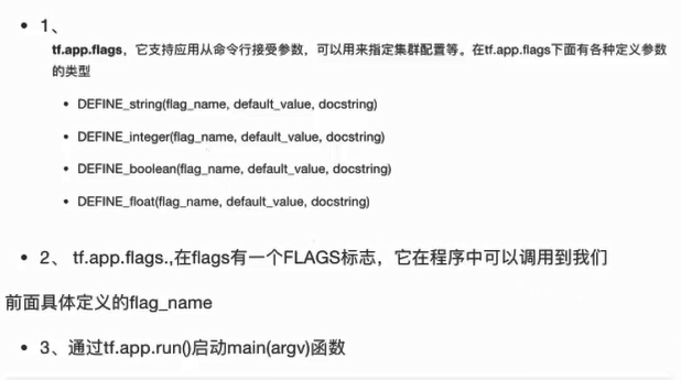
1.7.5 命令行参数的使用
import osimport tensorflow as tf2tf2.compat.v1.disable_eager_execution() tf = tf2.compat.v1.compat.v1 tf.app.flags.DEFINE_integer("max_step" , 100 , "训练模型的步数" ) tf.app.flags.DEFINE_string("model_dir" , "Unknown" , "模型保存的路径+模型名字" ) FLAGS = tf.app.flags.FLAGS def demo () : """ 命令行参数演示 :return: """ print("max_step:\n" , FLAGS.max_step) print("model_dir:\n" , FLAGS.model_dir) if __name__ == "__main__" : demo()
运行结果为
max_step:
 100
model_dir:
 Unknown
也可以使用以下命令启动,效果类似
python demo8.py --max_step=5 --model_dir="aaaa"
二 数据读取与神经网络 2.1 文件读取流程 有三种获取数据到TensorFlow程序中的方法
QueueRunner : 基于队列的输入管道从TensorFlow图形开始的文件中读取数据
Feeding : 运行每一步时 python 提供数据
预加载数据,TensorFlow图中的张量包含所有的数据(仅对于小数据集)
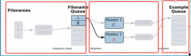
读取的步骤如下
1)构造文件名队列
file_queue = tf.train.string_input_producer(string_tensor,shuffle=True)
2)读取与解码
文本:
读取:tf.TextLineReader()
解码:tf.decode_csv()
图片:
读取:tf.WholeFileReader()
解码:
tf.image.decode_jpeg(contents)
tf.image.decode_png(contents)
二进制:
读取:tf.FixedLengthRecordReader(record_bytes)
解码:tf.decode_raw()
TFRecords
读取:tf.TFRecordReader()
key, value = 读取器.read(file_queue)
key:文件名
value:一个样本
3)批处理队列
tf.train.batch(tensors, batch_size, num_threads = 1, capacity = 32, name=None)
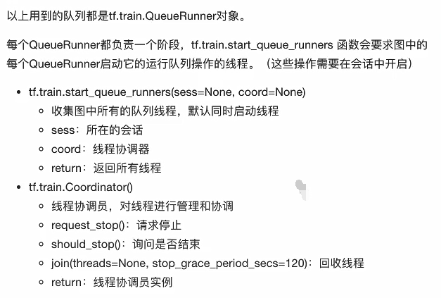
手动开启线程
tf.train.QueueRunner()
开启会话:
tf.train.start_queue_runners(sess=None, coord=None)
1 构造文件名队列
file_queue = tf.train.string_input_producer(string_tensor,shuffle=True ) string_tensor:含有文件名+路径的一阶张量 num_epochs : 过几遍数据,默认无线过数据 return 文件队列
2 读取与解码
阅读器默认每次只读取一个样本
文本文件默认一次读取一行,图片文件默认一次读取一张图片,二进制文件一次读取指定字节(最好是一个样本的字节数),TFRecords默认一次读取一个Example
tf.TextLineReader
阅读文本文件逗号分割值(CSV)格式,默认按行读取
return 读取器实例
tf.WholeFileReader : 用于读取图片文件
tf.FixedLengthRecordReader(record_bytes): 用于读取二进制文件
要读取每个记录是固定数量字节的二进制文件
record_bytes 整型,指定每次读取(一个样本的字节数),
return 读取器实例
tf.TFRecordReader :读取TFRecords文件
他们有共同的读取方法 read(file_queue) ,并且都会返回一个 tensor 元组。(key:文件名字,值:默认的内容,一个样本)
由于每次只会读取一个样本,所以如果要批处理需要使用tf.train.batch 或tf.train.shuffle_batch进行批处理操作,便于之后指定每批次多个样本的训练。
3 批处理
解码之后,可以直接获取默认的一个样本的内容了,但如果想要获取多个样本,需要加入到新的队列进行批处理。
tf.train.batch(tensors, batch_size, num_threads=1 , capacity=32 , enqueue_many=False , shapes=None , dynamic_pad=False , allow_smaller_final_batch=False , shared_name=None , name=None ) - 读取指定大小(个数)的张量 - tensors 可是包含张量的列表,批处理的内容放到列表之中 - batch_size 从队列中读取的批处理的大小 - num_threads 进入队列的线程数 - capacity 整数,队列中元素的最大数量 - return tensor
4 线程操作
2.2 图片数据读取 图片的基础知识
特征提取:
文本—- 数值(二维数组shape(n_samples,m_features))
字典—- 数值(二维数组shape(n_samples,m_features))
图片—- 数值(三维数组shape(图片长度,图片宽度,图片通道数))
组成图片的最基本单位是像素
图片三要素
灰度图 [长,宽,1] 每个像素点[0,255]的数
彩色图 [长,宽,3] 每个像素点用3个[0,255]的数
假设一张彩色图片的长200,宽200,通道数为3 ,那么总的像素数量为200 200 3
张量形状
一张图片可以表示为一个3D张量,即其形状为 [宽, 高, 通道数] ,其3D和4D的表示为
单个图片 [height, width, channel]
多个图片[batch,height, width, channel] batch表示一个批次的张量的数量
图片特征值处理
为什么要缩放图片到统一大小?
tf.image.resize_images(images, size) - 缩小放大图片 - images :4 -D形状[batch,height, width, channel]或3 -D形状 [height, width, channel]的张量的图片数据 - size :1 -D int32张量 :new_height,new_width 图片的新尺寸 - return 4 -D或3 -D格式图片
示例代码
import osimport tensorflow as tf2tf2.compat.v1.disable_eager_execution() tf = tf2.compat.v1.compat.v1 def demo () : """ 读取狗图片案例 :return: """ filename_list = os.listdir("./dog" ) file_list = [os.path.join("./dog/" , i) for i in filename_list] file_queue = tf.train.string_input_producer(file_list) reader = tf.WholeFileReader() key, value = reader.read(file_queue) print(f"key:{key} \n" ) print(f"value:{value} \n" ) image_decoded = tf.image.decode_jpeg(value) print(f"解码后的图片 :{image_decoded} \n" ) image_resized = tf.image.resize_images(image_decoded, [200 , 200 ]) print(f"缩放前的图片 :{image_resized} \n" ) image_resized.set_shape([200 , 200 , 3 ]) print(f"缩放后的图片 :{image_resized} \n" ) image_batch = tf.train.batch([image_resized], batch_size=100 , num_threads=2 , capacity=100 ) print(f"批处理队列 :{image_batch} \n" ) with tf.Session() as sess: coord = tf.train.Coordinator() threads = tf.train.start_queue_runners(sess=sess, coord=coord) filename, sample, image, n_image = sess.run([key, value, image_resized, image_batch]) print(f"filename:{filename} \n" ) print(f"sample:{sample} \n" ) print(f"image:{image} \n" ) print(f"n_image:{n_image} \n" ) coord.request_stop() coord.join(threads) if __name__ == "__main__" : demo()
运行结果为
key:Tensor("ReaderReadV2:0" , shape=(), dtype=string) value:Tensor("ReaderReadV2:1" , shape=(), dtype=string) 解码后的图片 :Tensor("DecodeJpeg:0" , shape=(None , None , None ), dtype=uint8) 缩放前的图片:Tensor("resize/Squeeze:0" , shape=(200 , 200 , None ), dtype=float32) 缩放后的图片 :Tensor("resize/Squeeze:0" , shape=(200 , 200 , 3 ), dtype=float32) 批处理队列 :Tensor("batch:0" , shape=(100 , 200 , 200 , 3 ), dtype=float32) filename:b'./dog/dog.95.jpg' sample:b'\xff\xd8\xff\xe0\x0...(这里省略全部输出打印) image:[[[ 2. 12. 13. ] [ 0. 10. 11. ] [ 0.9899998 8.99 10.99 ] ... 这里省略中间的输出 ... [34. 39. 42. ] [33. 38. 41. ] [35.504974 40.504974 43.504974 ]]] n_image:[[[[ 13. 14. 9. ] [ 13.99 14.99 9.99 ] [ 15.99 16.99 11.99 ] ... 这里省略中间的输出 ... [ 73.94 68.94 65.94 ] [ 72.23999 67.23999 64.23999 ] [ 71.140015 66.140015 63.140015 ]]]]
2.3 二进制数据读取 import osimport tensorflow as tf2tf2.compat.v1.disable_eager_execution() tf = tf2.compat.v1.compat.v1 class Cifar () : def __init__ (self) : self.height = 32 self.width = 32 self.channel = 3 self.image = self.height * self.width * self.channel self.label = 1 self.sample = self.image + self.label def read_binary (self) : """ 读取二进制文件 :return: """ filename_list = os.listdir("./cifar-10-batches-bin" ) file_list = [os.path.join("./cifar-10-batches-bin/" , i) for i in filename_list if i[-3 :] == "bin" ] file_queue = tf.train.string_input_producer(file_list) reader = tf.FixedLengthRecordReader(self.sample) key, value = reader.read(file_queue) image_decoded = tf.decode_raw(value, tf.uint8) print(f"图片解码 : {image_decoded} \n" ) label = tf.slice(image_decoded, [0 ], [self.label]) image = tf.slice(image_decoded, [self.label], [self.image]) print(f"标签 = :{label} \n" ) print(f"图片 = :{image} \n" ) image_reshaped = tf.reshape(image, [self.channel, self.height, self.width]) print(f"调整图像的形状 : {image_reshaped} \n" ) image_transposed = tf.transpose(image_reshaped, [1 , 2 , 0 ]) print(f"三维数组的转置 {image_transposed} :\n" ) image_batch, label_batch = tf.train.batch([image_transposed, label], batch_size=100 , num_threads=2 , capacity=100 ) with tf.Session() as sess: coord = tf.train.Coordinator() threads = tf.train.start_queue_runners(sess=sess, coord=coord) label_value, image_value = sess.run([label_batch, image_batch]) print(f"标签值 :{label_value} \n" ) print(f"图片:{image_value} \n" ) coord.request_stop() coord.join(threads) return image_value, label_value if __name__ == "__main__" : cifar = Cifar() cifar.read_binary()
运行结果为
图片解码 : Tensor("DecodeRaw:0" , shape=(None ,), dtype=uint8) 标签 = :Tensor("Slice:0" , shape=(1 ,), dtype=uint8) 图片 = :Tensor("Slice_1:0" , shape=(3072 ,), dtype=uint8) 调整图像的形状 : Tensor("Reshape:0" , shape=(3 , 32 , 32 ), dtype=uint8) 三维数组的转置 Tensor("transpose:0" , shape=(32 , 32 , 3 ), dtype=uint8): 标签值 :[[8 ] [3 ] [0 ] ****省略中间的输出 ***** [0 ] [7 ]] 图片:[[[[235 235 235 ] [231 231 231 ] ****省略中间的输出 ***** [199 178 127 ]]]]
2.4 TFRecords文件读取 import osimport tensorflow as tf2tf2.compat.v1.disable_eager_execution() tf = tf2.compat.v1.compat.v1 class Cifar () : def __init__ (self) : self.height = 32 self.width = 32 self.channel = 3 self.image = self.height * self.width * self.channel self.label = 1 self.sample = self.image + self.label def read_binary (self) : """ 读取二进制文件 :return: """ filename_list = os.listdir("./cifar-10-batches-bin" ) file_list = [os.path.join("./cifar-10-batches-bin/" , i) for i in filename_list if i[-3 :] == "bin" ] file_queue = tf.train.string_input_producer(file_list) reader = tf.FixedLengthRecordReader(self.sample) key, value = reader.read(file_queue) image_decoded = tf.decode_raw(value, tf.uint8) print(f"图片解码 : {image_decoded} \n" ) label = tf.slice(image_decoded, [0 ], [self.label]) image = tf.slice(image_decoded, [self.label], [self.image]) print(f"标签 = :{label} \n" ) print(f"图片 = :{image} \n" ) image_reshaped = tf.reshape(image, [self.channel, self.height, self.width]) print(f"调整图像的形状 : {image_reshaped} \n" ) image_transposed = tf.transpose(image_reshaped, [1 , 2 , 0 ]) print(f"三维数组的转置 {image_transposed} :\n" ) image_batch, label_batch = tf.train.batch([image_transposed, label], batch_size=100 , num_threads=2 , capacity=100 ) with tf.Session() as sess: coord = tf.train.Coordinator() threads = tf.train.start_queue_runners(sess=sess, coord=coord) label_value, image_value = sess.run([label_batch, image_batch]) print(f"标签值 :{label_value} \n" ) print(f"图片:{image_value} \n" ) coord.request_stop() coord.join(threads) return image_value, label_value def write_to_tfrecords (self, image_batch, label_batch) : """ 将样本的特征值和目标值一起写入tfrecords文件 :param image: :param label: :return: """ with tf.python_io.TFRecordWriter("cifar10.tfrecords" ) as writer: for i in range(100 ): image = image_batch[i].tostring() label = label_batch[i][0 ] example = tf.train.Example(features=tf.train.Features(feature={ "image" : tf.train.Feature(bytes_list=tf.train.BytesList(value=[image])), "label" : tf.train.Feature(int64_list=tf.train.Int64List(value=[label])), })) writer.write(example.SerializeToString()) return None def read_tfrecords (self) : """ 读取TFRecords文件 :return: """ file_queue = tf.train.string_input_producer(["cifar10.tfrecords" ]) reader = tf.TFRecordReader() key, value = reader.read(file_queue) feature = tf.parse_single_example(value, features={ "image" : tf.FixedLenFeature([], tf.string), "label" : tf.FixedLenFeature([], tf.int64) }) image = feature["image" ] label = feature["label" ] print("read_tf_image:\n" , image) print("read_tf_label:\n" , label) image_decoded = tf.decode_raw(image, tf.uint8) print("image_decoded:\n" , image_decoded) image_reshaped = tf.reshape(image_decoded, [self.height, self.width, self.channel]) print("image_reshaped:\n" , image_reshaped) image_batch, label_batch = tf.train.batch([image_reshaped, label], batch_size=100 , num_threads=2 , capacity=100 ) print("image_batch:\n" , image_batch) print("label_batch:\n" , label_batch) with tf.Session() as sess: coord = tf.train.Coordinator() threads = tf.train.start_queue_runners(sess=sess, coord=coord) image_value, label_value = sess.run([image_batch, label_batch]) print("image_value:\n" , image_value) print("label_value:\n" , label_value) coord.request_stop() coord.join(threads) return None if __name__ == "__main__" : cifar = Cifar() image_value, label_value = cifar.read_binary() cifar.write_to_tfrecords(image_value, label_value) cifar.read_tfrecords()
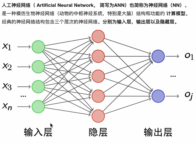
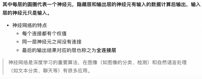
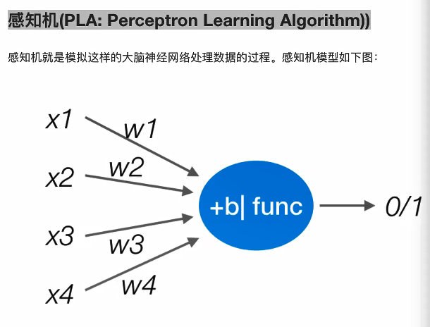
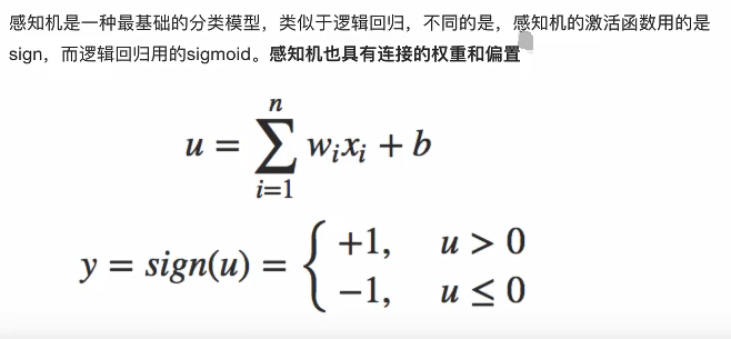
2.5 神经元网络
神经网络的主要用途是用作分类,在使用的过程中,主要是围绕 损失、优化这两款来进行的。
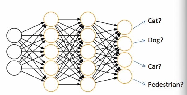
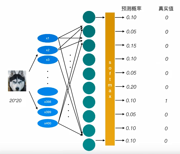
神经网络解决多分类问题最常用的方法是设置n个输出节点,其中n为类别的个数。
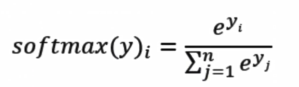
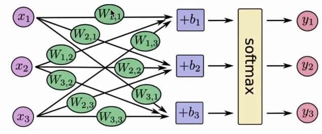
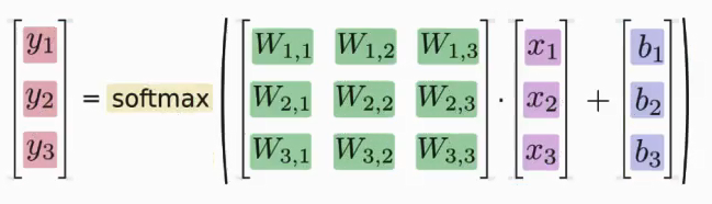
2.5.1 softmax回归 softmax回归将神经网络输出转换成概率结果
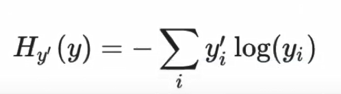
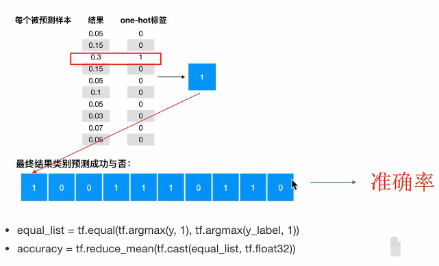
2.5.2 交叉熵损失
为了衡量距离,目标值需要进行one-hot,能与概率值一一对应,如下图
损失大小
神经网络最后的损失为平均每个样本的损失大小
对所有样本的损失求和取其平均值
训练过程中计算器会尝试一点点增加或减小每个参数,看其能如何减少相比于训练数据集的误差,以望能找到最优的权重和偏置参数组合。
计算 labels 和 logits 之间的交叉损失熵
tf.nn.softmax_cross_entropy_with_logits(labels=None , logits=None , name=None ) labels :标签值(真实值) logits : 样本加权之后的值 return 返回损失值列表
计算张量的尺寸的元素平均值
tf.reduce_min(input_tensor)
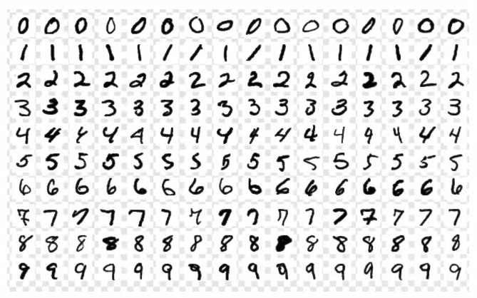
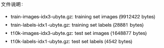
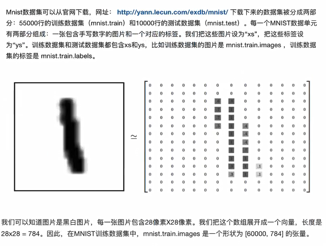
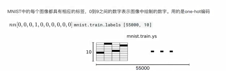
2.6 案例:使用全连接对手写数字识别 2.6.1 数据集介绍
参考网站 (lecun.com)
特征值
目标值
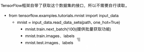
mnist数据获取API
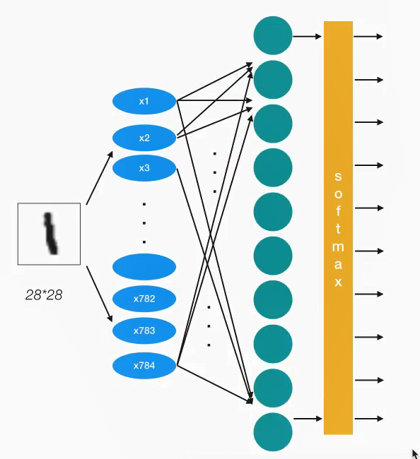
2.6.2 基本使用 1 网络设计
我们采用一层即最后一个输出层的神经网格,也称之为全连接层神经网络
2 全连接层计算
计算全连接结果,供交叉损失运算
tf.matmul(a, b, name=None ) +bias return 全连接结果,供交叉损失运算
梯度下降
tf.train.GradientDescentOptimizer(learning_rate)

learning_rate : 学习率

方法
	minimize :最小优化损失
import tensorflow as tffrom tensorflow.examples.tutorials.mnist import input_datadef full_connection () : """ 用全连接对手写数字进行识别 :return: """ mnist = input_data.read_data_sets("./mnist_data" , one_hot=True ) X = tf.placeholder(dtype=tf.float32, shape=[None , 784 ]) y_true = tf.placeholder(dtype=tf.float32, shape=[None , 10 ]) weights = tf.Variable(initial_value=tf.random_normal(shape=[784 , 10 ], stddev=0.01 )) bias = tf.Variable(initial_value=tf.random_normal(shape=[10 ], stddev=0.1 )) y_predict = tf.matmul(X, weights) + bias loss_list = tf.nn.softmax_cross_entropy_with_logits(logits=y_predict, labels=y_true) loss = tf.reduce_mean(loss_list) optimizer = tf.train.AdamOptimizer(learning_rate=0.01 ).minimize(loss) bool_list = tf.equal(tf.argmax(y_true, axis=1 ), tf.argmax(y_predict, axis=1 )) accuracy = tf.reduce_mean(tf.cast(bool_list, tf.float32)) init = tf.global_variables_initializer() with tf.Session() as sess: sess.run(init) for i in range(5000 ): image, label = mnist.train.next_batch(500 ) _, loss_value, accuracy_value = sess.run([optimizer, loss, accuracy], feed_dict={X: image, y_true: label}) print("第%d次的损失为%f,准确率为%f" % (i+1 , loss_value, accuracy_value)) return None if __name__ == "__main__" : full_connection()
2.6.3 完善功能模型 计算准确率
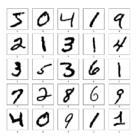
2.7 基于tensorflow2的mnist识别 2.7.1 准备数据 import tensorflow as tfimport numpy as npimport matplotlib as mplimport matplotlib.pyplot as plt(train_images, train_labels), (test_images, test_labels) = tf.keras.datasets.mnist.load_data() print("train_images shape" , train_images.shape) train_images = train_images / 255.0 test_images = test_images / 255.0 plt.figure(figsize=(10 , 10 )) for i in range(25 ): plt.subplot(5 , 5 , i + 1 ) plt.xticks([]) plt.yticks([]) plt.grid(False ) plt.imshow(train_images[i], cmap=plt.cm.binary) plt.xlabel(train_labels[i]) plt.show()
显示出图像
2.7.2 完整代码 import tensorflow as tfimport numpy as npdef prepare () : (train_images, train_labels), (test_images, test_labels) = tf.keras.datasets.mnist.load_data() train_images, test_images = train_images / 255.0 , test_images / 255.0 return train_images, test_images, train_labels, test_labels def exec () : model = tf.keras.Sequential([ tf.keras.layers.Flatten(input_shape=(28 , 28 )), tf.keras.layers.Dense(128 , activation='relu' ), tf.keras.layers.Dense(10 , activation='softmax' ) ]) model.compile(optimizer='adam' , loss='sparse_categorical_crossentropy' , metrics=['acc' ]) return model if __name__ == "__main__" : train_images, test_images, train_labels, test_labels = prepare() model = exec() model.fit(train_images, train_labels, epochs=10 ) test_loss, test_acc = model.evaluate(test_images, test_labels, verbose=2 ) print(f'当前损失值为 {test_loss} ,准确值为 {test_acc} ' ) predictions = model.predict(test_images) print('预测值:' , np.argmax(predictions[0 ])) print('真实值:' , test_labels[0 ])
运行结果为
Epoch 1 /10 1875 /1875 [==============================] - 2 s 717 us/step - loss: 0.2576 - acc: 0.9252 Epoch 2 /10 1875 /1875 [==============================] - 1 s 696 us/step - loss: 0.1108 - acc: 0.9669 Epoch 3 /10 1875 /1875 [==============================] - 1 s 717 us/step - loss: 0.0767 - acc: 0.9773 Epoch 4 /10 1875 /1875 [==============================] - 1 s 712 us/step - loss: 0.0556 - acc: 0.9827 Epoch 5 /10 1875 /1875 [==============================] - 1 s 692 us/step - loss: 0.0444 - acc: 0.9863 Epoch 6 /10 1875 /1875 [==============================] - 1 s 715 us/step - loss: 0.0345 - acc: 0.9895 Epoch 7 /10 1875 /1875 [==============================] - 1 s 653 us/step - loss: 0.0273 - acc: 0.9915 Epoch 8 /10 1875 /1875 [==============================] - 1 s 699 us/step - loss: 0.0214 - acc: 0.9936 Epoch 9 /10 1875 /1875 [==============================] - 1 s 696 us/step - loss: 0.0187 - acc: 0.9944 Epoch 10 /10 1875 /1875 [==============================] - 1 s 654 us/step - loss: 0.0160 - acc: 0.9951 313 /313 - 0 s - loss: 0.0730 - acc: 0.9796 当前损失值为 0.07301463931798935 ,准确值为 0.9796000123023987 预测值: 7 真实值: 7
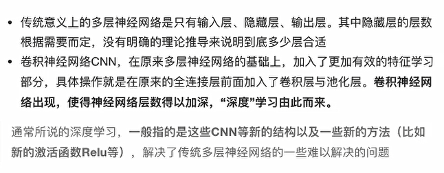
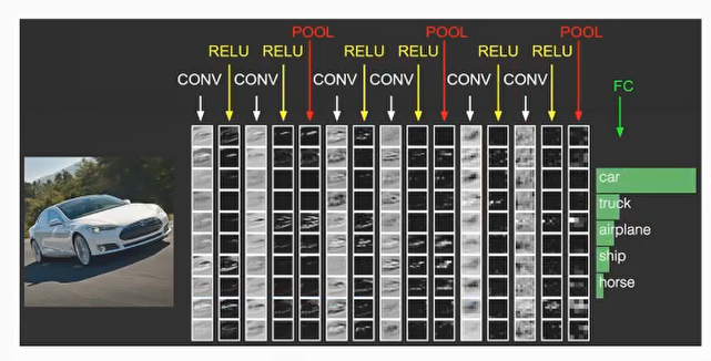
三 卷积神经网络 卷积神经网络与传统多层神经网络的对比
3.1 卷积神经网络的三个结构
神经网络的基本组成包含 输入层、隐藏层、输出层,而卷积神经网络的特点在于隐藏层分为卷积层和池化层(pooling layer,又叫下采样层)以及激活层,每层的作用如下
卷积层:通过在原始图像上平移来提取特征
激活层:增加非线性切割能力
池化层: 减少学习的参数,降低网络负责度(最大池化和平均池化)
为了达到分类效果,还有一个全连接层(Full Connection),也就是最后的输出层,进行损失计算并输出分类结果。
3.2 卷积层
卷积神经网络中每层卷积层由若干卷积单元(卷积核)组成 ,每个卷积单元的参数都是 通过反向传播算法最佳化得到的。
卷积运算的目的是特征提取,第一层卷积层可能只能提取一些低级的特征如边缘、线条和角等层级,更多层的网络能从低级特征中迭代提取更复杂的特征。
卷积核(Filter)的四大要素
卷积核个数
卷积核大小
卷积核步长
卷积核零填充大小
接下来通过案例计算讲解,假设图片都是黑白图片(只有一个通道)
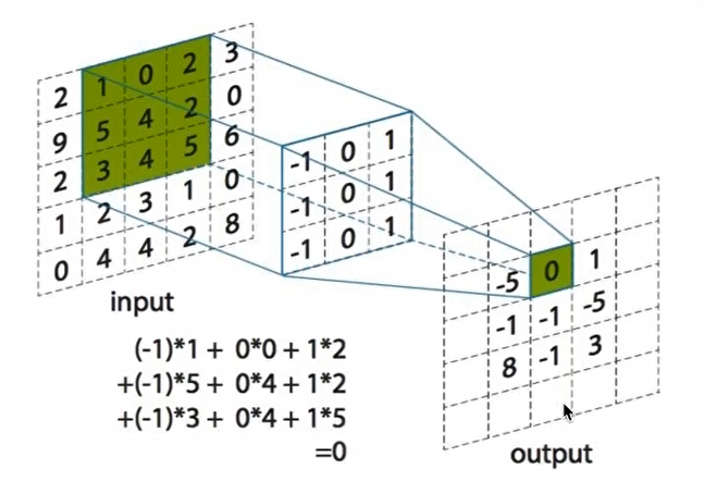
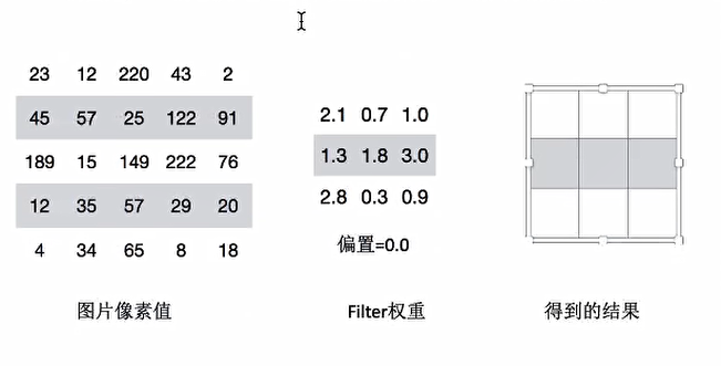
3.2.1 卷积如何计算大小 卷积核我们可以理解为一个观察的人,带着若干权重和一个偏置去观察,进行特征加权运算。
注:上述要加上偏置
卷积核大小 : 1 1 、3 3、5 * 5
通过卷积核选择这些大小,是经过研究人员经过实验证明比较好的结果,这个人观察之后就会得到一个运算结果
        输入
            5*5*1 filter 3*3*1 步长 1
        输出
            3*3*1
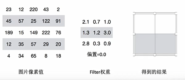
如果这个需要观察这个图片所有的像素,只需要平移即可。
3.2.2 卷积计算步长 平移卷积核观察这个图片,需要的参数就是步长
假设移动步长是一个像素,那么最终这个人观察的的结果以下图为例
5 5的图片,3 3 的卷积大小去1个步长运算得到 3 * 3 的大小观察结果
如果步长为2 ,那么结果是这样
5 5的图片,3 3 的卷积大小去2个步长运算得到 3 * 3 的大小观察结果
3.2.3 卷积核个数的计算 如果在某一层结构中,不止一个人观察,多个人(卷积核)一起观察,那就得到多个观察结果
不同卷积核带的权重和偏置都不一样,即随机初始化的参数
输出的结果处理由大小和步长决定外,还会被零填充影响。
Filter观察窗口的大小和移动步长有时会导致超过图片像素宽度。
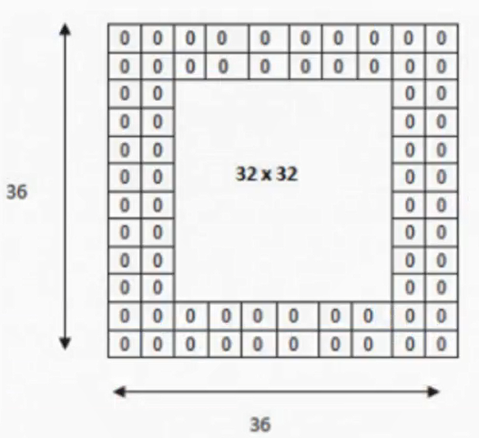
3.2.4 卷积计算零填充大小 零填充就是在图片像素外围填充一圈值为0的像素
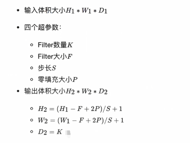
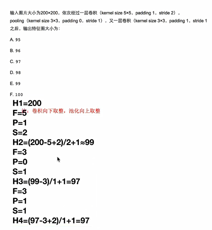
如果已知输入图片形状,卷积核数量,卷积核大小,以及移动步长,那么输出图片形状为
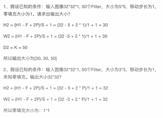
计算案例如下
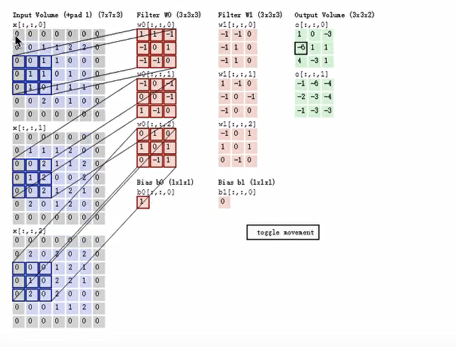
3.2.5 多通道图片如何观察 如果是一张彩色图片,那么就有三种表分别为R,G,B。原本每个人需要带一个3x3 或者其他大小的卷积核,现在需要带3张3x3的权重和一个偏量,总共就27个权重。最终每个人还是得出一张结果:
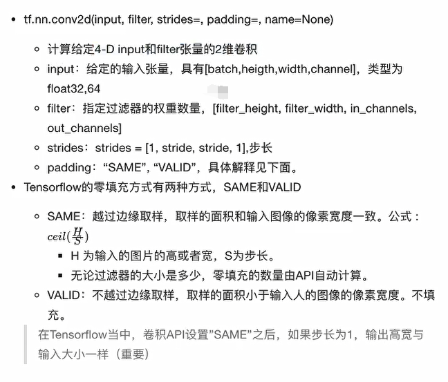
3.2.6 卷积网络API
3.3 激活函数 随着神经网络的发展,大家发现原有的sigmoid等激活函数并不能达到好的效果,所以采用新的激活函数。
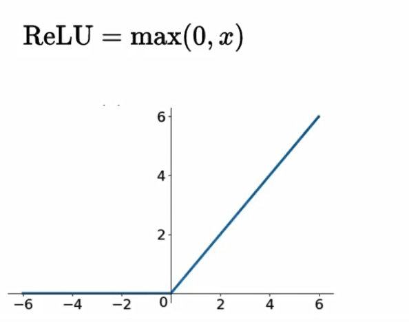
3.3.1 Relu
3.3.2 playground演示不同激活函数作用
具体参见 http://playground.tensorflow.org
3.3.3 为什么采用新的激活函数
Relu优点
有效解决梯度消失问题
计算速度非常快,只需要判断输入是否大于0。SGD(批梯度下降)的求解速度远快于sigmoid和tanh
sigmoid缺点
采用sigmoid等函数,计算量相对大,而采用Relu激活函数,整个过程的计算量节省很多。在深层网络中,sigmoid函数反向传播时,很容易就会出现梯度消失的情况
3.3.4 激活函数API tf.nn.relu(features, name=None ) features : 卷积后加上偏置的结果 return : 结果
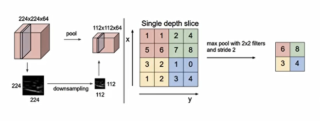
3.4 池化层 pooling 层的主要作用是特征提取,通过去掉Feature Map中不重要的样本,进一步减少参数数量。Pooling的方法很多,通吃采用最大池化
max_polling : 取池化窗口的最大值
avg_polling : 取池化窗口的平均值
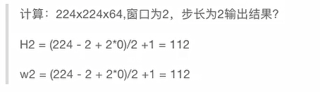
3.4.1 池化层计算 池化层也有窗口的大小和移动步长,其计算公式通卷积计算公式一致
通常池化采用 2 * 2 大小,步长为2的窗口
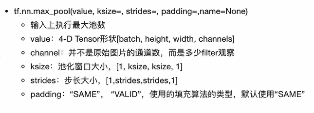
3.4.2 池化层API
3.5 全连接层 前面卷积核池化相当于做特征工程,最后的全连接层在整个卷积神经网络中起到“分类器”的作用
3.6 案例:CNN-Mnist手写数字识别 import tensorflow as tfimport osfrom tensorflow.examples.tutorials.mnist import input_datafrom tensorflow.contrib.slim.python.slim.nets.inception_v3 import inception_v3_basetf.app.flags.DEFINE_integer("is_train" , 1 , "指定是否是训练模型,还是拿数据去预测" ) FLAGS = tf.app.flags.FLAGS def create_weights (shape) : return tf.Variable(initial_value=tf.random_normal(shape=shape, stddev=0.01 )) def create_model (x) : """ 构建卷积神经网络 :param x: :return: """ with tf.variable_scope("conv1" ): input_x = tf.reshape(x, shape=[-1 , 28 , 28 , 1 ]) conv1_weights = create_weights(shape=[5 , 5 , 1 , 32 ]) conv1_bias = create_weights(shape=[32 ]) conv1_x = tf.nn.conv2d(input=input_x, filter=conv1_weights, strides=[1 , 1 , 1 , 1 ], padding="SAME" ) + conv1_bias relu1_x = tf.nn.relu(conv1_x) pool1_x = tf.nn.max_pool(value=relu1_x, ksize=[1 , 2 , 2 , 1 ], strides=[1 , 2 , 2 , 1 ], padding="SAME" ) with tf.variable_scope("conv2" ): conv2_weights = create_weights(shape=[5 , 5 , 32 , 64 ]) conv2_bias = create_weights(shape=[64 ]) conv2_x = tf.nn.conv2d(input=pool1_x, filter=conv2_weights, strides=[1 , 1 , 1 , 1 ], padding="SAME" ) + conv2_bias relu2_x = tf.nn.relu(conv2_x) pool2_x = tf.nn.max_pool(value=relu2_x, ksize=[1 , 2 , 2 , 1 ], strides=[1 , 2 , 2 , 1 ], padding="SAME" ) with tf.variable_scope("full_connection" ): x_fc = tf.reshape(pool2_x, shape=[-1 , 7 * 7 * 64 ]) weights_fc = create_weights(shape=[7 * 7 * 64 , 10 ]) bias_fc = create_weights(shape=[10 ]) y_predict = tf.matmul(x_fc, weights_fc) + bias_fc return y_predict def full_connected_mnist () : """ 单层全连接神经网络识别手写数字图片 特征值:[None, 784] 目标值:one_hot编码 [None, 10] :return: """ mnist = input_data.read_data_sets("./mnist_data/" , one_hot=True ) with tf.variable_scope("mnist_data" ): x = tf.placeholder(tf.float32, [None , 784 ]) y_true = tf.placeholder(tf.int32, [None , 10 ]) y_predict = create_model(x) with tf.variable_scope("softmax_crossentropy" ): loss = tf.reduce_mean(tf.nn.softmax_cross_entropy_with_logits(labels=y_true, logits=y_predict)) with tf.variable_scope("optimizer" ): train_op = tf.train.AdamOptimizer(0.001 ).minimize(loss) with tf.variable_scope("accuracy" ): equal_list = tf.equal(tf.argmax(y_true, 1 ), tf.argmax(y_predict, 1 )) accuracy = tf.reduce_mean(tf.cast(equal_list, tf.float32)) tf.summary.scalar("losses" , loss) tf.summary.scalar("acc" , accuracy) init_op = tf.global_variables_initializer() merged = tf.summary.merge_all() saver = tf.train.Saver() with tf.Session() as sess: sess.run(init_op) file_writer = tf.summary.FileWriter("./tmp/summary/" , graph=sess.graph) if FLAGS.is_train == 1 : for i in range(3000 ): mnist_x, mnist_y = mnist.train.next_batch(50 ) sess.run(train_op, feed_dict={x: mnist_x, y_true: mnist_y}) print("训练第%d步的准确率为:%f, 损失为:%f " % (i+1 , sess.run(accuracy, feed_dict={x: mnist_x, y_true: mnist_y}), sess.run(loss, feed_dict={x: mnist_x, y_true: mnist_y}) ) ) summary = sess.run(merged, feed_dict={x: mnist_x, y_true: mnist_y}) file_writer.add_summary(summary, i) else : for i in range(100 ): mnist_x, mnist_y = mnist.test.next_batch(1 ) print("第%d个样本的真实值为:%d, 模型预测结果为:%d" % ( i+1 , tf.argmax(sess.run(y_true, feed_dict={x: mnist_x, y_true: mnist_y}), 1 ).eval(), tf.argmax(sess.run(y_predict, feed_dict={x: mnist_x, y_true: mnist_y}), 1 ).eval() ) ) return None if __name__ == "__main__" : full_connected_mnist()
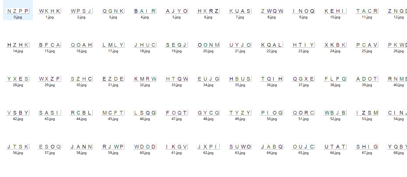
3.7 案例:验证码识别 3.7.1 原始的图片数据和标签值 一共有6000张验证码图片,标签值为验证码图片包含的4个字母,以图片文件名为索引放在labels.csv文件中。
3.7.2 读取图片数据 按照文件读取流程进行读取,和之前的区别在于读取器同时返回了文件名和图片内容,文件名会一并返回作为查询具体的标签值的索引。
import globimport tensorflow as tf2tf2.compat.v1.disable_eager_execution() tf = tf2.compat.v1.compat.v1 def read_picture () : """ 读取验证码图片 :return: """ file_list = glob.glob("./GenPics/*.jpg" ) print(f"文件列表 = :{file_list} \n" ) file_queue = tf.train.string_input_producer(file_list) print(f"文件队列为 = :{file_queue} \n" ) reader = tf.WholeFileReader() filename, image = reader.read(file_queue) print(f"读取后的文件名为 = :{filename} \n" ) print(f"读取后的图片为 = :{image} \n" ) image_decode = tf.image.decode_jpeg(image) image_decode.set_shape([20 , 80 , 3 ]) print(f"解码后的图片为 = : {image_decode} \n" ) image_cast = tf.cast(image_decode, tf.float32) filename_batch, image_batch = tf.train.batch([filename, image_cast], batch_size=100 , num_threads=2 , capacity=100 ) print(f"返回数据中的 filename_batch 为 = : {filename_batch} \n" ) print(f"返回数据中的 image_batch 为 = : {image_batch} \n" ) return filename_batch, image_batch if __name__ == "__main__" : read_picture()
输出结果为
文件列表 = :['./GenPics\\0.jpg' ,...省略中间的输出...'./GenPics\\999.jpg' ] 文件队列为 = :<tensorflow.python.ops.data_flow_ops.FIFOQueue object at 0x000001251C46CB20 > 读取后的文件名为 = :Tensor("ReaderReadV2:0" , shape=(), dtype=string) 读取后的图片为 = :Tensor("ReaderReadV2:1" , shape=(), dtype=string) 解码后的图片为 = : Tensor("DecodeJpeg:0" , shape=(20 , 80 , 3 ), dtype=uint8) 返回数据中的 filename_batch 为 = : Tensor("batch:0" , shape=(100 ,), dtype=string) 返回数据中的 image_batch 为 = : Tensor("batch:1" , shape=(100 , 20 , 80 , 3 ), dtype=float32)
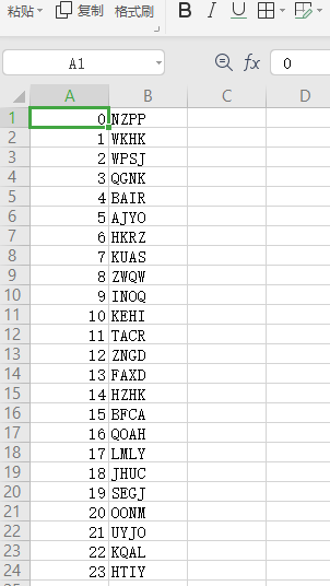
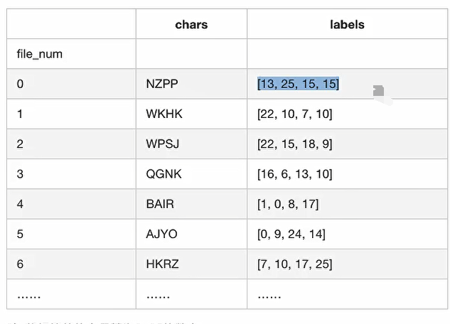
3.7.3 文件名与标签值对应 解析csv文件,建立文件名与标签值对应表格
import pandas as pdimport tensorflow as tf2tf2.compat.v1.disable_eager_execution() tf = tf2.compat.v1.compat.v1 def parse_csv () : csv_data = pd.read_csv("./GenPics/labels.csv" , names=["file_num" , "chars" ], index_col="file_num" ) labels = [] for label in csv_data["chars" ]: print(f" label = {label} \n" ) tmp = [] for letter in label: tmp.append(ord(letter) - ord("A" )) labels.append(tmp) print(f" labels = {labels} \n" ) csv_data["labels" ] = labels return csv_data if __name__ == "__main__" : csv_data = parse_csv() print(f" csv_data = \n {csv_data} " )
输出结果为
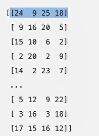
3.7.4 标签值字母转换成数字 将标签值的字母转换成0 ~ 25的数字
训练中读取每个图片时会获得每个图片的文件名,需要得到对应的标签值数据
def filename2label (filenames, csv_data) : """ 将filename和标签值联系起来 :param filenames: :param csv_data: :return: """ labels = [] for filename in filenames: digit_str = "" .join(list(filter(str.isdigit, str(filename)))) label = csv_data.loc[int(digit_str), "labels" ] labels.append(label) return np.array(labels)
得到的结果为
3.7.5 建立卷积神经网络模型 模型的结构与之前的mnist手写字识别是一样的,由两个卷积层和全连接输出层组成
def create_weights (shape) : return tf.Variable(initial_value=tf.random_normal(shape=shape, stddev=0.01 )) def create_model (x) : """ 构建卷积神经网络 :param x:[None, 20, 80, 3] :return: """ with tf.variable_scope("conv1" ): conv1_weights = create_weights(shape=[5 , 5 , 3 , 32 ]) conv1_bias = create_weights(shape=[32 ]) conv1_x = tf.nn.conv2d(input=x, filter=conv1_weights, strides=[1 , 1 , 1 , 1 ], padding="SAME" ) + conv1_bias relu1_x = tf.nn.relu(conv1_x) pool1_x = tf.nn.max_pool(value=relu1_x, ksize=[1 , 2 , 2 , 1 ], strides=[1 , 2 , 2 , 1 ], padding="SAME" ) with tf.variable_scope("conv2" ): conv2_weights = create_weights(shape=[5 , 5 , 32 , 64 ]) conv2_bias = create_weights(shape=[64 ]) conv2_x = tf.nn.conv2d(input=pool1_x, filter=conv2_weights, strides=[1 , 1 , 1 , 1 ], padding="SAME" ) + conv2_bias relu2_x = tf.nn.relu(conv2_x) pool2_x = tf.nn.max_pool(value=relu2_x, ksize=[1 , 2 , 2 , 1 ], strides=[1 , 2 , 2 , 1 ], padding="SAME" ) with tf.variable_scope("full_connection" ): x_fc = tf.reshape(pool2_x, shape=[-1 , 5 * 20 * 64 ]) weights_fc = create_weights(shape=[5 * 20 * 64 , 4 * 26 ]) bias_fc = create_weights(shape=[104 ]) y_predict = tf.matmul(x_fc, weights_fc) + bias_fc return y_predict
3.7.6 完整代码实现 流程分析
import globimport pandas as pdimport numpy as npimport tensorflow as tf2tf2.compat.v1.disable_eager_execution() tf = tf2.compat.v1.compat.v1 def read_picture () : """ 读取验证码图片 :return: """ file_list = glob.glob("./GenPics/*.jpg" ) file_queue = tf.train.string_input_producer(file_list) reader = tf.WholeFileReader() filename, image = reader.read(file_queue) image_decode = tf.image.decode_jpeg(image) image_decode.set_shape([20 , 80 , 3 ]) image_cast = tf.cast(image_decode, tf.float32) filename_batch, image_batch = tf.train.batch([filename, image_cast], batch_size=100 , num_threads=2 , capacity=100 ) return filename_batch, image_batch def parse_csv () : csv_data = pd.read_csv("./GenPics/labels.csv" , names=["file_num" , "chars" ], index_col="file_num" ) labels = [] for label in csv_data["chars" ]: tmp = [] for letter in label: tmp.append(ord(letter) - ord("A" )) labels.append(tmp) csv_data["labels" ] = labels return csv_data def filename2label (filenames, csv_data) : """ 将filename和标签值联系起来 :param filenames: :param csv_data: :return: """ labels = [] for filename in filenames: digit_str = "" .join(list(filter(str.isdigit, str(filename)))) label = csv_data.loc[int(digit_str), "labels" ] labels.append(label) return np.array(labels) def create_weights (shape) : return tf.Variable(initial_value=tf.random_normal(shape=shape, stddev=0.01 )) def create_model (x) : """ 构建卷积神经网络 :param x:[None, 20, 80, 3] :return: """ with tf.variable_scope("conv1" ): conv1_weights = create_weights(shape=[5 , 5 , 3 , 32 ]) conv1_bias = create_weights(shape=[32 ]) conv1_x = tf.nn.conv2d(input=x, filter=conv1_weights, strides=[1 , 1 , 1 , 1 ], padding="SAME" ) + conv1_bias relu1_x = tf.nn.relu(conv1_x) pool1_x = tf.nn.max_pool(value=relu1_x, ksize=[1 , 2 , 2 , 1 ], strides=[1 , 2 , 2 , 1 ], padding="SAME" ) with tf.variable_scope("conv2" ): conv2_weights = create_weights(shape=[5 , 5 , 32 , 64 ]) conv2_bias = create_weights(shape=[64 ]) conv2_x = tf.nn.conv2d(input=pool1_x, filter=conv2_weights, strides=[1 , 1 , 1 , 1 ], padding="SAME" ) + conv2_bias relu2_x = tf.nn.relu(conv2_x) pool2_x = tf.nn.max_pool(value=relu2_x, ksize=[1 , 2 , 2 , 1 ], strides=[1 , 2 , 2 , 1 ], padding="SAME" ) with tf.variable_scope("full_connection" ): x_fc = tf.reshape(pool2_x, shape=[-1 , 5 * 20 * 64 ]) weights_fc = create_weights(shape=[5 * 20 * 64 , 4 * 26 ]) bias_fc = create_weights(shape=[104 ]) y_predict = tf.matmul(x_fc, weights_fc) + bias_fc return y_predict def exec () : filename, image = read_picture() csv_data = parse_csv() x = tf.placeholder(tf.float32, shape=[None , 20 , 80 , 3 ]) y_true = tf.placeholder(tf.float32, shape=[None , 4 * 26 ]) y_predict = create_model(x) loss_list = tf.nn.sigmoid_cross_entropy_with_logits(labels=y_true, logits=y_predict) loss = tf.reduce_mean(loss_list) optimizer = tf.train.AdamOptimizer(learning_rate=0.001 ).minimize(loss) equal_list = tf.reduce_all( tf.equal(tf.argmax(tf.reshape(y_predict, shape=[-1 , 4 , 26 ]), axis=2 ), tf.argmax(tf.reshape(y_true, shape=[-1 , 4 , 26 ]), axis=2 )), axis=1 ) accuracy = tf.reduce_mean(tf.cast(equal_list, tf.float32)) init = tf.global_variables_initializer() with tf.Session() as sess: sess.run(init) coord = tf.train.Coordinator() threads = tf.train.start_queue_runners(sess=sess, coord=coord) for i in range(1000 ): filename_value, image_value = sess.run([filename, image]) labels = filename2label(filename_value, csv_data) labels_value = tf.reshape(tf.one_hot(labels, depth=26 ), [-1 , 4 * 26 ]).eval() _, error, accuracy_value = sess.run([optimizer, loss, accuracy], feed_dict={x: image_value, y_true: labels_value}) print("第%d次训练后损失为%f,准确率为%f" % (i + 1 , error, accuracy_value)) coord.request_stop() coord.join(threads) if __name__ == "__main__" : exec()
运行结果为
第1次训练后损失为1.674498,准确率为0.000000
第2次训练后损失为0.909409,准确率为0.000000
第3次训练后损失为0.266742,准确率为0.000000
第4次训练后损失为0.177306,准确率为0.000000
***************************